Learning Geometric Shapes with a Multi-layer Perceptron

Download the Source Code for this Post

For this post, we will look at how a Multi-layer Perceptron learns data by looking at how it learns simple geometric shapes.

We will be using the standard logistic activation function, logistic(x) = 1 / (1 + exp(-x)), or in python:

# Define Logistic Function
def logistic(x):
    return 1 / (1 + np.exp(-x))

Here is a graph of the logistic function:

Graph of Logistic Function

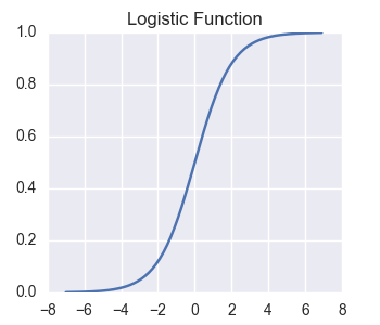
As you can see, the logistic function flattens out for values far from zero.

However, we will be looking at functions of two variables f(x,y). So our Multi-Layer Perceptron will be structured similar to the following figure: Picture of Example Multi-Layer Perceptron Model

Now, let’s set up our x-values and y-values in 2d arrays.

# Set up domain value arrays.
X = np.arange(100)[np.newaxis, :]
X = np.full((100, 100), X, dtype = 'float32')

Y = np.arange(100)[::-1, np.newaxis]
Y = np.full((100, 100), Y, dtype = 'float32')

Now, let’s set up a logistic function for 2d variables that really only depends on x. We also give it an offset by 50 in the x-direction.

 def f(x, y):
    return logistic(x - 50) 

Now let’s take a look at its graph as a heat map. We will be using the module seaborn and call it by the standard convention sns.

import seaborn as sns

Now print out the heat map.

z = f(X, Y) 

plt.clf()
xticks = np.arange(0, 100, 10)
yticks = np.arange(0, 100, 10)
ax = sns.heatmap(z, vmin = 0.0, vmax = 1.0, xticklabels = xticks, yticklabels = yticks[::-1]) 
ax.set_xticks(xticks)
ax.set_yticks(yticks)

Picture of One Logistic

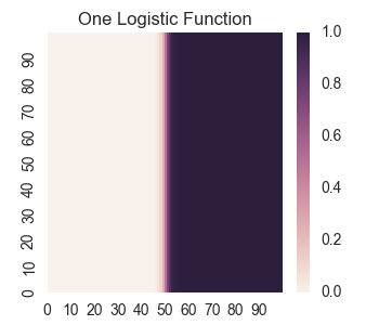
Note that we are graphing from x = 0 to x = 100, and at this scale, the graph of looks like a sharp transition from 0 to 1 at x = 50.

Manual Combinations of Logistic Functions

First let’s set up our different logistic functions.

def layer1_node1(x, y):
    return logistic(-x +  35)
def layer1_node2(x, y):
    return logistic(y - 65)
def layer1_node3(x, y):
    return logistic(x - 65)
def layer1_node4(x, y):
    return logistic(-y + 35)

Now let’s consider taking the average of two logistic functions.

z = 1/2.0 * layer1_node2(X,Y) + 1/2.0 * layer1_node3(X,Y) 

plt.clf()
ax = sns.heatmap(z, vmin = 0.0, vmax = 1.0, xticklabels = xticks, yticklabels = yticks[::-1]) 
ax.set_xticks(xticks)
ax.set_yticks(yticks)
plt.title('Two Logistic Functions')
plt.savefig('2017-10-17-graphs/manual_twolog.png')

Picture of Two Logistics

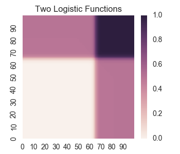
Here we observe a problem for using simple combinations of logistic functions (i.e. one hidden layer). They are incapable of learning a simple bounded geometric object; that is, the combination must be non-desirable values outside the shape. For example, let’s try combining four logistic functions to make a square.

z = 0.5 * layer1_node1(X,Y) + 0.5 * layer1_node2(X,Y) + 0.5 * layer1_node3(X,Y) + 0.5 * layer1_node4(X,Y)

plt.clf()
ax = sns.heatmap(z, vmin = 0.0, vmax = 1.0, xticklabels = xticks, yticklabels = yticks[::-1]) 
ax.set_xticks(xticks)
ax.set_yticks(yticks)
plt.title('Four Logistic Functions')
plt.savefig('2017-10-17-graphs/manual_fourlog.png')

Picture of Four Logistics

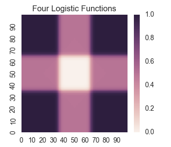
What we want is a square of 0 values in the center and all other values are close to 1. However, we see that there are large sections outside the square where we get other values. To fix this, we will need to add another hidden layer.

Manually Adding a Second Hidden Layer

Now let’s consider what happends when we manually add in a second hidden layer. First let’s look at learning a corner shape. Before when we looked at a combination of two logistic functions, we had values outside the corner that weren’t the desired value of 1. Now we may compose this (and an additional offset and scaling) with a logistic function to force all values outside the corner to be 1.

def layer2_node1(x, y):
    result = layer1_node2(X,Y) + layer1_node3(X,Y) - 1/2
    return logistic( result * 10)

z = layer2_node1(X,Y) 
plt.clf()
ax = sns.heatmap(z, vmin = 0.0, vmax = 1.0, xticklabels = xticks, yticklabels = yticks[::-1]) 
ax.set_xticks(xticks)
ax.set_yticks(yticks)
plt.title('Hidden Layer Sizes is (2, 1)')
plt.savefig('2017-10-17-graphs/manual_hidden(2,1).png')

Picture of Corner with Manual Two Hidden Layers

We can also do something similar to obtain a square.

def layer2_node2(x, y):
    result = layer1_node1(X,Y) + layer1_node2(X,Y) + layer1_node3(X,Y) + layer1_node4(X,Y) - 1/2
    return logistic( result * 10)

z = layer2_node2(X, Y)
plt.clf()
ax = sns.heatmap(z, vmin = 0.0, vmax = 1.0, xticklabels = xticks, yticklabels = yticks[::-1]) 
ax.set_xticks(xticks)
ax.set_yticks(yticks)
plt.title('Hidden Layer Sizes is (4, 1)')
plt.savefig('2017-10-17-graphs/manual_hidden(4,1).png')

Picture of Square with Manual Two Hidden Layers

In fact, we can now construct more complicated shapes. For example, we can make another larger square and then subtract it from our previous square.

def layer1_node5(x, y):
    return logistic(-x +  25)
def layer1_node6(x, y):
    return logistic(y - 75)
def layer1_node7(x, y):
    return logistic(x - 75)
def layer1_node8(x, y):
    return logistic(-y + 25)

def layer2_node3(x, y):
    result = layer1_node5(X,Y) + layer1_node6(X,Y) + layer1_node7(X,Y) + layer1_node8(X,Y) - 1/2
    return logistic(result * 10)

z = -layer2_node3(X,Y) + layer2_node2(X,Y) 
plt.clf()
ax = sns.heatmap(z, vmin = 0.0, vmax = 1.0, xticklabels = xticks, yticklabels = yticks[::-1]) 
ax.set_xticks(xticks)
ax.set_yticks(yticks)
plt.title('Hidden Layer Sizes is (8, 2)')
plt.savefig('2017-10-17-graphs/manual_hidden(8,2).png')

Picture of Complex Square with Manual Two Hidden Layers

Now, let’s take a look at using scikit-learn’s MLPRegressor() to actually try to learn these shapes.

Learning a Square with MLPRegressor()

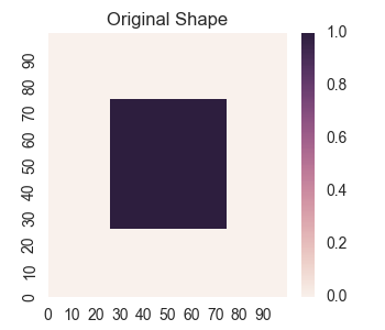
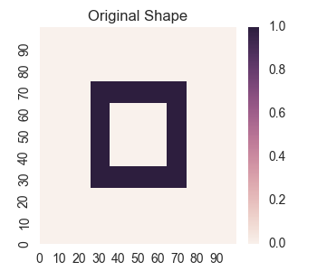
We will look at learning the square for various sizes of hidden layers. First, let’s construct the original square we will use to teach our model.

# Construct a mask for the square
mask = (25 < X) & (X < 75) & (25 < Y) & (Y < 75)
z = np.zeros(X.shape)
z[mask] = 1.0
plt.clf()
ax = sns.heatmap(z, vmin = 0.0, vmax = 1.0, xticklabels = xticks, yticklabels = yticks[::-1]) 
ax.set_xticks(xticks)
ax.set_yticks(yticks)
plt.title('Original Shape')
plt.savefig('2017-10-17-graphs/square_train.png')

Picture of Original Square

For sci-kit learn’s MLPRegressor(), the sizes are stored in the parameter hidden_layer_sizes. Also, note that we need to apply a StandardScaler() to the data to pre-process it before feeding it to the neural network, and we have manually adjusted the initial learning rate to give overall good performance for the layer sizes we are trying.

hidden_layer_sizes = [(1), (2), (3), (4), (10), (100), (5, 2), (8, 2), (10, 10), (10, 10, 10), (10, 10, 10, 10)]
X_train = np.stack([X.reshape(-1), Y.reshape(-1)], axis = -1)
y_train = z.reshape(-1)
mlp = MLPRegressor( activation = 'logistic',
                    learning_rate_init = 1e-1,
                    random_state = 2017 )
model = Pipeline([ ('scaler', StandardScaler()),
                   ('mlp', MLPRegressor( activation = 'logistic',
                                         learning_rate_init = 1e-1,
                                         random_state = 2017 ) ) ])

for sizes in hidden_layer_sizes:
    model.set_params(mlp__hidden_layer_sizes = sizes)
    model.fit(X_train, y_train)
    y_predict = model.predict(X_train)
    z_predict = y_predict.reshape(X.shape)
    plt.clf()
    ax = sns.heatmap(z_predict, vmin = 0.0, vmax = 1.0, xticklabels = xticks, yticklabels = yticks[::-1]) 
    ax.set_xticks(xticks)
    ax.set_yticks(yticks)
    plt.title('hidden_layer_sizes = ' + str(sizes))
    plt.savefig('2017-10-17-graphs/square' + str(sizes) + '.png')
    print('Finished ', sizes)

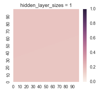
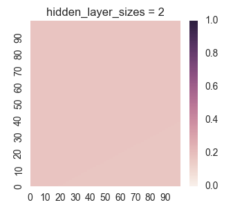
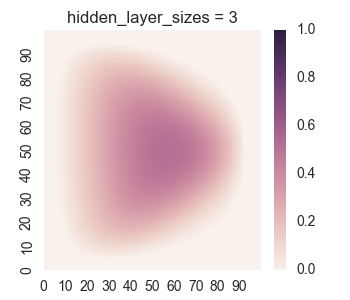
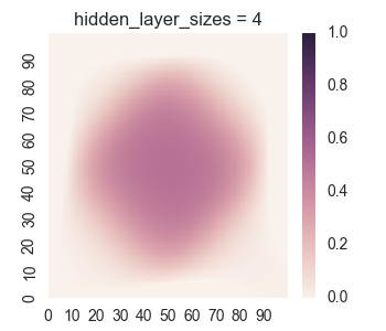
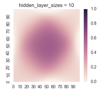
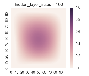
First let’s take a look at the results for only one hidden layer.

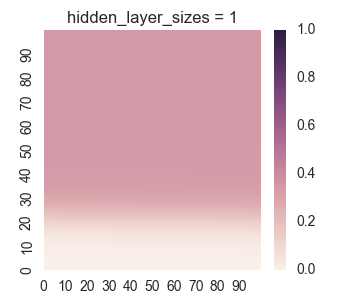
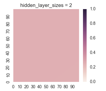
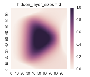
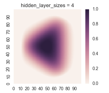
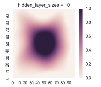
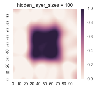
Picture Learning Square for Layer Sizes = (1)

We see that the picture looks reasonable only for a large number of nodes if there is only one hidden layer. Furthermore, we can see undersirable values bleeding out of the square into the surrounding region, as we discussed when we were manually looking at a single layer. Now let’s take a look at the results for two hidden layers.

Picture Learning Square for Layer Sizes = (5, 2)

We see that for hidden_layer_sizes = (5, 2), the learned shape is a blurry and warped square. This is in contrast to the result we had when we manually could get the square for a size of (4, 2). There are a couple things to take into consideration. First, sci-kit learn’s MLPRegressor() controls the size of the coefficient it finds by using a regularity penalty. After applying a standard scaling, the set up from the manual set up would require very large coefficients. One can see this from the fact that the almost instant transition from 0 to 1 would require very large derivatives.

Second, of course, is that the algorithm won’t perfectly learn the shape, as its optimal function isn’t convex in the coefficients.

Now let’s see the results for three and four layers.

Picture Learning Square for Layer Sizes = (10, 10, 10)

We see that there isn’t really any improvement over using just two layers.

Learning the More Complex Square Shape with MLPRegressor()

Now let’s try learning the more complex square shape with sci-kit learn’s MLPRegressor(). Let’s set up the shape we will use for training.

mask = (25 < X) & (X < 75) & (25 < Y) & (Y < 75)
mask2 = (35 < X) & (X < 65) & (35 < Y) & (Y < 65)
z = np.zeros(X.shape)
z[mask & ~mask2] = 1.0
plt.clf()
ax = sns.heatmap(z, vmin = 0.0, vmax = 1.0, xticklabels = xticks, yticklabels = yticks[::-1]) 
ax.set_xticks(xticks)
ax.set_yticks(yticks)
plt.title('Original Shape')
plt.savefig('2017-10-17-graphs/annular_train.png')

Picture of Original Complex Square For Training

Now, let’s try learning this shape with sci-kit learn’s MLPRegressor().

y_train = z.reshape(-1)
model = Pipeline([ ('scaler', StandardScaler()),
                   ('mlp', MLPRegressor(hidden_layer_sizes = (3),
                                        activation = 'logistic',
                                        learning_rate_init = 1e-1,
                                        random_state = 2017) ) ])
                                        
for sizes in hidden_layer_sizes:
    model.set_params(mlp__hidden_layer_sizes = sizes)
    model.fit(X_train, y_train)
    y_predict = model.predict(X_train)
    z_predict = y_predict.reshape(X.shape)

    plt.clf()
    ax = sns.heatmap(z_predict, vmin = 0.0, vmax = 1.0, xticklabels = xticks, yticklabels = yticks[::-1]) 
    ax.set_xticks(xticks)
    ax.set_yticks(yticks)
    plt.title('hidden_layer_sizes = ' + str(sizes))
    plt.savefig('2017-10-17-graphs/annular' + str(sizes) + '.png')
    print('Finished ', sizes)

Let’s take a look at the results for one hidden layer.

Picture of Complex Square for Hidden Layer Sizes = (1)

We see that the results for one hidden layer aren’t very good, which isn’t very surprising. It is near impossible for just logistic functions to create the empty region between the square regions. Now let’s take a look at the results for two hidden layers.

Picture of Complex Square for Hidden Layer Sizes = (5,2)

Despite the fact that in the manual case, we did a very good job for a hidden layer size of (8, 2), we see that the learning algorithm does not do a good job. However a hidden layer size of (10, 10) does a decent job, but there is still some bleeding of values seen in the bottom region. Now let’s look at the results for three and four hidden layers.

Picture of Complex Square for Hidden Layer Sizes = (10, 10, 10)

Again, the results for more layers isn’t really any better than two layers.

Varying Regularity For Many Nodes

Now let’s take a look at the effect of varying the L2 regularization penalty for a network of three hidden layers with sizes (50, 50, 50). It is often recommended to train on varying the regularization strength versus training on the layer sizes, for example see these notes for Stanford’s Neural Network course. For sklearn’s MLPRegressor, the regularity in the fitted parameters is controlled by the hyper-parameter alpha.

model = Pipeline([ ('scaler', StandardScaler()),
                   ('mlp', MLPRegressor(hidden_layer_sizes = (50, 50, 50),
                           activation = 'logistic',
                           learning_rate_init = 1e-1,
                           random_state = 2017) ) ])
alphas = [1e-1, 1e-2, 1e-3, 1e-4, 1e-5, 1e-6]

for alpha, i in zip(alphas, range(len(alphas))):
    model.set_params(mlp__alpha = alpha)
    model.fit(X_train, y_train)
    y_predict = model.predict(X_train)
    z_predict = y_predict.reshape(X.shape)

    plt.clf()
    ax = sns.heatmap(z_predict, vmin = 0.0, vmax = 1.0, xticklabels = xticks, yticklabels = yticks[::-1]) 
    ax.set_xticks(xticks)
    ax.set_yticks(yticks)
    plt.title('alpha = ' + str(alpha))
    plt.savefig('2017-10-17-graphs/annular_regularity' + str(i) + '.png')
    print('Finished ', alpha)

We get the following results:

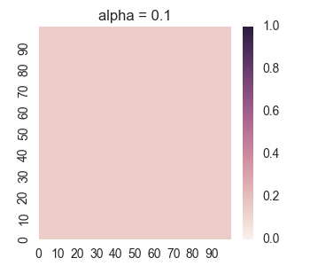
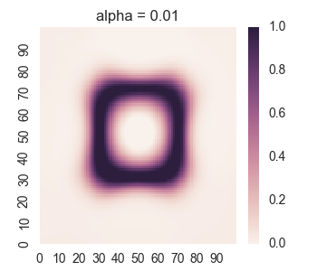
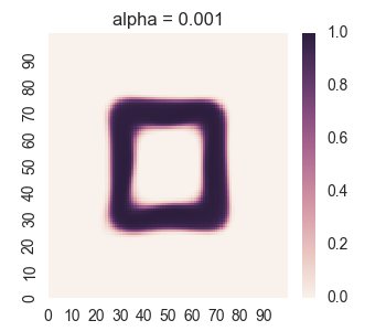
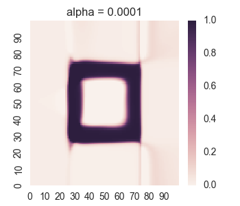
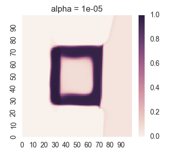
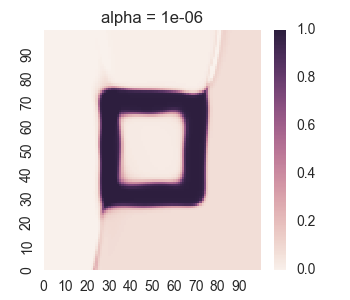
Picture For Regularity alpha0 Picture For Regularity alpha1 Picture For Regularity alpha2 Picture For Regularity alpha3 Picture For Regularity alpha4 Picture For Regularity alpha5

For too much regularity, i.e. alpha = 0.1, we don’t get convergence. For too little regularity, e.g. alpha = 1e-6, we get bleeding of values to the region outside of the geometric shape.