Download the Source Code for This Post
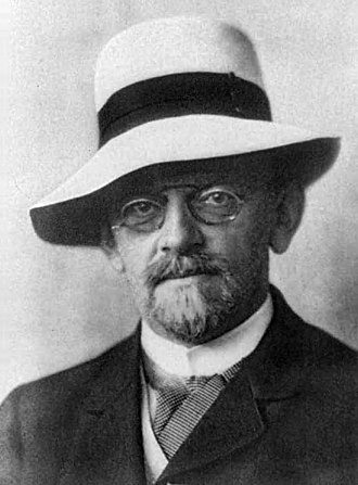
In this post, we will be using tensorflow to try to create a cartoon effect on a picture; unfortunately, we will come up short and only create an interesting shading effect. We will take a picture of the mathematician David Hilbert and consider the pixel values to be a function of the two coordinates x and y. Then we will try to use a multi-layer perceptron regressor to create a more simplified representation of the image. The predicted image of this neural network will be too smooth, so we will simplify the colors to a palette of 8 possible shades of grey.
Pictured below is the result.

Note that in the interest of saving memory, we have made the effects images smaller than the original. This can easily be adjusted in the source code by changing:
fig = plt.figure(figsize = (3.5,3))
So why use a neural network? The idea is that neural networks in theory can learn the output of complicated functions, but in practice won’t learn them in complete detail. This is especially true if we put in restrictions such as those related to the regularity of coefficients.
Before continuing our discussion, let’s load the modules we will need for this project.
import tensorflow as tf
import numpy as np
import matplotlib.pyplot as plt
import seaborn as sns
from PIL import Image
Simple Palette Reduction is Still Too Real
Now you might be wondering “Why not just take the original image and restrict to say a palette of 8 shades of grey?” The problem with this approach is that the result will look too real and have too much detail. Let’s take a look. First, here is the code to load the image, reduce the color palette, and save the result:
# Open the image we will try to turn into a cartoon.

img = Image.open('HilbertPic.jpg')
img = np.asarray(img, dtype = 'int32')
print('img.shape = ', img.shape)

# Function for plotting images with tick marks.

def plotimage(data):
    nY, nX = data.shape
    plt.clf()
    plt.imshow(data, cmap = plt.get_cmap('gray'))
    labels = np.arange(0, 1, .1)
    yticks = np.arange(0, 1, .1)
    ax = plt.gca()
    ax.grid(False)
    plt.xticks(np.arange(0, nX, nX / 10), labels)
    plt.yticks(np.arange(0, nY, nY / 10), 1.0 - labels)


# Function to turn image into an image of discrete number of grayscale levels.

def stratify(X, levels):
    nLevels = len(levels)
    X[X < levels[0]] = levels[0]
    for i in range(nLevels - 1):
        mask = (X > levels[i]) & (X < levels[i+1])
        X[mask] = levels[i]
    X[X > levels[nLevels - 1]] = levels[nLevels - 1]
    return X

stratlevels = np.arange(0, 256, int(256 / 8))
stratimg = stratify(img, stratlevels)

plotimage(stratimg)
plt.title('Simple Discrete Levels')
plt.savefig('2017-10-30-graphs/simple.png')
Now let’s take a look at the results of this simple procedure.
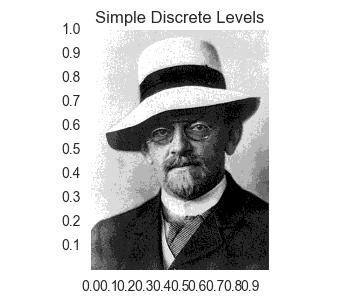
As you can see, this is still a pretty realistic picture and not what we are looking for.
First Attempt Using Tensorflow
Now let’s try to use tensorflow to construct a multi-layer perceptron to learn the image. First let’s create our features for prediction, which for now are simply the x and y values of each pixel.
# Set up features for X and Y coordinates.

nY, nX = img.shape
X = np.full(img.shape, np.arange(nX))
X = X / nX
Y = np.full(img.shape, np.arange(nY)[:, np.newaxis])
Y = nY - 1 - Y
Y = Y / nY

img = img.reshape(-1, 1)
print('img.shape = ', img.shape)

# First let's just try learning the picture using the X and Y coordinates as features.

features = np.concatenate([X.reshape(-1, 1), Y.reshape(-1, 1)], axis = -1)

nSamples, nFeatures = features.shape
print('features.shape = ', features.shape)
Now, let’s set up the layers inside our multi-layer perceptron. We will need to do this more than once, so we will create a function to do; the function will have a parameter for the number of features since we will add a feature in a later section. Our function will return a dictionary of references to certain weights and tensorflow graph nodes that we will need layer.
# Set up layers.

print('Setting up layers.')

tf.set_random_seed(20171026)
np.random.seed(20171026)

def createLayers(nFeatures):

    init_stddev = 0.5
    init_mean = 0.0
    init_bias = 0.1
    hidden1size = 50
    hidden2size = 50
    hidden3size = 50

    x = tf.placeholder(tf.float32, shape = [None, nFeatures])
    y_ = tf.placeholder(tf.float32, shape = [None, 1])

    W1 = tf.Variable(tf.truncated_normal([nFeatures, hidden1size], stddev = init_stddev, mean = init_mean) )
    b1 = tf.Variable(tf.zeros([hidden1size]) + init_bias)
    hidden1 = tf.nn.relu(tf.matmul(x, W1) + b1)

    W2 = tf.Variable(tf.truncated_normal([hidden1size, hidden2size], stddev = init_stddev, mean = init_mean))
    b2 = tf.Variable(tf.zeros([hidden2size]) + init_bias)
    hidden2 = tf.nn.relu(tf.matmul(hidden1, W2) + b2)

    W3 = tf.Variable(tf.truncated_normal([hidden2size, hidden3size], stddev = init_stddev, mean = init_mean))
    b3 = tf.Variable(tf.zeros([hidden3size]) + init_bias)
    hidden3 = tf.nn.relu(tf.matmul(hidden2, W3) + b3)

    Wout = tf.Variable(tf.truncated_normal([hidden3size, 1], stddev = init_stddev, mean = init_mean))
    bout = tf.Variable(tf.zeros([1]) + init_bias)
    out = tf.matmul(hidden3, Wout) + bout

    layers = { 'x':x, 'y_':y_, 'W1':W1, 'out':out }
    return layers

layers = createLayers(nFeatures)
Now, let’s set up the loss function and the training step.
# Set up the loss function and training step.

print('Setting up loss.')

l2_loss = tf.reduce_mean(tf.square(layers['out'] - layers['y_']))
train_step = tf.train.AdamOptimizer(1e-2).minimize(l2_loss)
Now let’s train our network on the image and get a result. First, let’s create a generic function for running our training session that returns the result and loss training information.
batchsize = 200

def runSession(nsteps):
    with tf.Session() as sess:

        sess.run(tf.global_variables_initializer())

        losses = []
        losses_index = []
        for i in range(nsteps):
            batchi = np.random.randint(0, len(img), size = batchsize)
            batchx = features[batchi]
            batchy = img[batchi]
            sess.run(train_step, {layers['x']: batchx, layers['y_']: batchy})
            if i % 100 == 0:
                newloss = sess.run(l2_loss, {layers['x']: features, layers['y_']: img})
                losses.append(newloss)
                losses_index.append(i)
                print(i, ' loss = ', newloss)

        result = sess.run(layers['out'], {layers['x']: features})

        return losses_index, losses, result
Finally, let’s train the network and view both the training losses and the final result.
print('\nTraining for Constant Rate')
losses_index, losses, result = runSession(10000)

plt.clf()
plt.plot(losses_index[1:], losses[1:])
plt.title('Losses for Constant Training Rate')
plt.savefig('2017-10-30-graphs/constantRateLosses.svg')

result = result.reshape(nY, nX)
plotimage(result)
plt.title('Constant Training Rate')
plt.savefig('2017-10-30-graphs/constantRate.png')
Here is the graph of the losses and the final result.

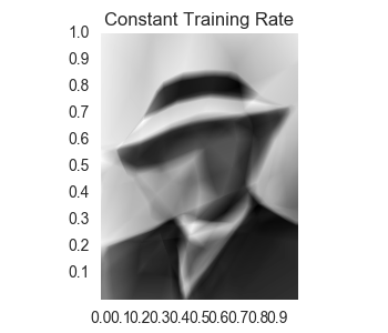
As we can see, the result of the neural network is too smooth. Let’s rough it up by reducing its color palette to 8 shades of grey.
result[result > 255] = 255
result[result < 0] = 0
stratlevels = np.arange(0, 256, int(256 / 8))
result = stratify(result, stratlevels)
plotimage(result)
plt.title('Constant Rate After Stratifying')
plt.savefig('2017-10-30-graphs/constantRateStrat.png')
We get

Second Attempt: Decaying Training Rate
Now, let’s try to recover more detail on the face by adding a decay to our training rate. We need to redefine our training step.
global_step = tf.Variable(0, trainable = False)
learning_rate_init = 1e-1
learning_rate = tf.train.exponential_decay(learning_rate_init, global_step, 500, 10**(-1/20 * 1.50), staircase = True)

train_step = tf.train.AdamOptimizer(learning_rate).minimize(l2_loss, global_step = global_step)
Now, let’s train the network and get the result.
print('\nTraining for Variable Training Rate')
losses_index, losses, result = runSession(10000)

plt.clf()
plt.plot(losses_index[1:], losses[1:])
plt.title('Losses for Decaying Training Rate')
plt.savefig('2017-10-30-graphs/decayRateLosses.svg')

result = result.reshape(nY, nX)
plotimage(result)
plt.title('Decaying Training Rate')
plt.savefig('2017-10-30-graphs/decayRate.png')
We get:


Now, we can see that we have a better detection of the outline of the left side of the face; however the facial details aren’t really any more clear. Let’s see what this looks like when we reduce the color palette.

Third Attempt: Add a Feature for Neighborhood Standard Deviation
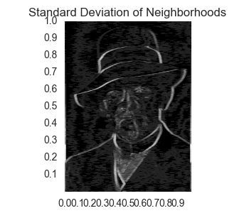
To try to get more detail on the face, let’s try adding another feature. Currently, we have a sample for every x and y position in the image, i.e. for every pixel. For each of these pixels, our new feature will be a standard deviation of the pixels that occur in a neighborhood of the pixel.
First, we construct a function to get the neighbors of each pixel. For simplicity, the pixels on the edges will have copies of edge pixels for those pixels in the neighborhood that don’t actually occur in the image. After we have the neighboring pixels, we find the standard deviation. Furthermore, we normalize the standard deviation feature to be between 0 and 1. The neighborhood will be constructed with a certain size that was found to provide good results by trial and error.
# Now look at creating another feature based on standard deviation in neighborhood of point.

def getNeighborhood(X, nbrRadius):
    rowsX, colsX = X.shape
    cols = np.arange(-nbrRadius, nbrRadius + 1)[np.newaxis, :]
    rows = np.arange(-nbrRadius, nbrRadius + 1)[:, np.newaxis]
    cols = np.arange(colsX)[np.newaxis, :, np.newaxis, np.newaxis] + cols
    rows = np.arange(rowsX)[:, np.newaxis, np.newaxis, np.newaxis] + rows
    cols = np.amax([cols, np.zeros(cols.shape)], axis = 0)
    rows = np.amax([rows, np.zeros(rows.shape)], axis = 0)
    cols = np.amin([cols, np.full(cols.shape, colsX - 1)], axis = 0)
    rows = np.amin([rows, np.full(rows.shape, rowsX - 1)], axis = 0)
    rows = rows.astype('int32')
    cols = cols.astype('int32')

    nbrs = X[rows, cols]
    nbrs = nbrs.reshape(rowsX, colsX, -1)
    rowsX, colsX, nNbrs = nbrs.shape
    nbrs = nbrs.reshape(-1, nNbrs)
    return nbrs

nbrs = getNeighborhood(img, 4)
print('nbrs.shape = ', nbrs.shape)

nbrs = nbrs.std(axis = -1, keepdims = True)
nbrs = nbrs / np.amax(nbrs)
We can print out this neighborhood feature as a picture.
plotimage(nbrs.reshape(nY, nX))
plt.title('Standard Deviation of Neighborhoods')
plt.savefig('2017-10-30-graphs/nbrFeature.png')
We get the following result:
Okay, now let’s create the new features.
# Create new features.

features = np.concatenate([X.reshape(-1, 1), Y.reshape(-1, 1), nbrs.reshape(-1,1)], axis = -1)

nSamples, nFeatures = features.shape
print('features.shape = ', features.shape)
We need to recreate our layers, our loss function, training rate, and training step.
# Recreate layers.

print('Setting up layers.')
tf.reset_default_graph()
tf.set_random_seed(20171026)
np.random.seed(20171026)

layers = createLayers(nFeatures)

# Set up loss.

print('Setting up loss.')

l2_loss = tf.reduce_mean(tf.square(layers['out'] - layers['y_']))

global_step = tf.Variable(0, trainable = False)
learning_rate_init = 1e-1
learning_rate = tf.train.exponential_decay(learning_rate_init, global_step, 500, 10**(-1/20 * 1.50), staircase = True)

train_step = tf.train.AdamOptimizer(learning_rate).minimize(l2_loss, global_step = global_step)
Now let’s train the model and get the results.
print('Training for Including Neighborhood Stddev')
losses_index, losses, result = runSession(10000)

plt.clf()
plt.plot(losses_index[1:], losses[1:])
plt.title('Losses for Including Neighborhood Stddev')
plt.savefig('2017-10-30-graphs/nbrLosses.svg')

result = result.reshape(nY, nX)
plotimage(result)
plt.title('Using Neighborhood Stddev')
plt.savefig('2017-10-30-graphs/nbr.png')
We get:

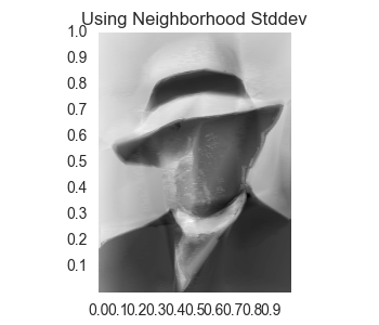
So we see that there is now some ugly noise in the face of the prediction. Let’s take a look at what this looks like when we reduce the color palette.
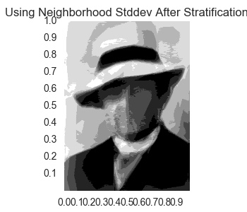 The noise is still there and creates more of an effect that looks more creepy than what we desire.
Last Attempt: Put Some Regularity on the Neighbor Feature
Let’s keep the neighborhood standard deviation feature we added in the last section, but let’s add a regularizer based on the weights for this feature in the first hidden layer. This will allow the model to use this feature, but reduce its effect to allow the noise to be smoothed out. So let’s set up our regularizer and create a new loss function. We will also need to recreate some of the other parts of our model.
print('Setting up loss.')

l2_reg = tf.contrib.layers.l2_regularizer(scale = 10**1.5)
reg_term = tf.contrib.layers.apply_regularization(l2_reg, weights_list = [layers['W1'][2, :]])
l2_loss = tf.reduce_mean(tf.square(layers['out'] - layers['y_'])) + reg_term

global_step = tf.Variable(0, trainable = False)
learning_rate_init = 1e-1
learning_rate = tf.train.exponential_decay(learning_rate_init, global_step, 500, 10**(-1/20 * 1.50), staircase = True)

train_step = tf.train.AdamOptimizer(learning_rate).minimize(l2_loss, global_step = global_step)
Now let’s train the model and get the results.
print('Training for Regularity Applied to Neighborhood Feature')
losses_index, losses, result = runSession(10000)

plt.clf()
plt.plot(losses_index[1:], losses[1:])
plt.title('Losses for Using Regularity Neighborhood Stddev')
plt.savefig('2017-10-30-graphs/regularityLosses.svg')

result = result.reshape(nY, nX)
plotimage(result)
plt.title('Using Regularity of Neighborhood Stddev')
plt.savefig('2017-10-30-graphs/regularity.png')
We get:

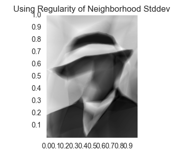
It seems we have some outline of the nose and part of the beard. Let’s look at what happens when we reduce the palette.
So we have several different results. We have certainly fallen short of creating a “cartoonification” of the original image. Furthermore, it really seems which is preferable is a matter of personal preference. No method is so outperforming of the other to call a clear winner.