Download the Source Code For This Post
In this post we will explore using solutions to the travelling salesman problem to create images that are drawn with a single closed curve; for a true solution to the travelling salesman problem, this curve will not cross itself. However, we will be using the method of simulated annealing to find approximate solutions to the travelling salesman problem. So our curves will have some self-crossings, but the number of crossings shouldn’t be too large.
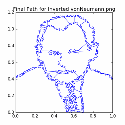
This post is inspired by the travelling salesman art created by others, such as the art at Professor Bosch’s webpage. For example, the following applying our method to a simple tracing of a portrait of John Von Neumann:
The overview of our method is two steps:
- Use random sampling to sample pixels where the probability density is within a normalization factor given by the intensity of each pixel. This sampling can be accomplished with simple rejection sampling. The samples we obtain will be the vertices of our travelling salesman problem.
- Try to find approximate solutions to the travelling salesman problem for our vertices. That is, we try to find a closed tour of our vertices of minimal length.
We implement both of these steps in the classes
RejectionSamplerandAnnealingTSP.
First, we will give a small discussion of the travelling salesman problem and then simulated annealing for the travelling salesman problem. A nice discussion of applying simulated annealing to the travelling salesman problem is given in the article The Evolution of Markov Chain Monte Carlo Methods by Matthew Richey.
Then we will show examples of using the classes RejectionSampler and AnnealingTSP. Finally we will discuss the implementation details of these classes.
Before we get started, let’s look at the modules we will need to import for our code:
import numpy as np
import matplotlib.pyplot as plt
from PIL import Image # Necessary for opening images inorder to sample their pixels.
import io # Used for itermediary when saving pyplot figures as PNG files so that we can use PIL
          # to reduce the color palette; this reduces file size.
Also let’s set up a seed to numpy.random in order to get consistent results:
# Set up a random seed for consistent results.

np.random.seed(20180327)
The Travelling Salesman Problem
The travelling salesman problem, as we will use it, is simply that we have a list of vertices and we wish to find a closed circuit (i.e. a cycle) that visits each vertex exactly once and is of minimal length. The name comes from the idea that the problem represents the optimal way a travelling salesman can visit a list of cities.
Ultimately our goal is really to construct images using a continuous, closed, non-self-intersecting curve. A true solution to the travelling salesman problem should provide this as it can’t cross itself. Unfortunately, our method of simulated annealing should really only be expected to give approximate solutions. So we will still have self-intersections, but their number should be small(ish).
Simulated Annealing for the Travelling Salesman Problem
Simulated annealing tries to randomly find a minimum for an energy function by imitating the statistical nature of a thermodynamic system undergoing cooling. Again, I would like to mention the article The Evolution of Markov Chain Monte Carlo Methods by Matthew Richey.
We randomly explore the state space using a random walk very similar to that in the Metropolis method of sampling. Let us discuss what this means for the travelling salesman problem.
For the travelling salesman problem, our states are the different possible cycles; these can alternatively be understood to be the different possible orderings of our vertices (i.e. what order do we visit them). The energy function will simply be the length of the current cycle.
How should we walk around our space of possible states? The idea is that we can reach any permutation through a sequence of flipping the order of continuous chains. This is best explained
through example. Consider the case of six vertices denoted by V[0], V[1], …, and V[5] as in the picture below:

We randomly select two indices i and j to be the endpoints of the chain that we wish to flip. We don’t explicitly require i < j. For example, in the next picture we have
selected i = 1 and j = 3. Now there is a small catch as the chain “between” V[i] and V[j] could be either V[1], V[2], V[3] or V[3], V[4], V[5], V[0], V[1]. However,
which one we select to change doesn’t change the effect on the length of the cycle. In fact, there is an even stronger statement that there is a symmetry between
all of the possible later moves from either decision. We won’t go into any detail, but the point is that it doesn’t matter which we choose. We choose V[1], V[2], V[3] as circled in the
following picture:

Then we make a flip of the chain V[1], V[2], V[3]. That is the old V[1] becomes the new V[3], and the old V[3] becomes the new V[1]:

Notice the source of the change in the cycle length is only coming from our endpoints V[i] and V[j] switching one of their neighbors. This is great news, because
it means we can calculate how the length (i.e. energy) changes by only working with V[i], V[j], and their neighbors. We don’t need to do calculations for the entire
cycle. In more technical terms, we can find the change in length using an O(1) operation instead of a O(N) operation.
Now, for simulated annealing, we don’t always accept such proposed moves. How we accept these proposed flips is given by the following rules:
- If the length decreases, then the move is accepted and the flip occurs.
- Else if the length increases, then we randomly accept the move with probability
np.exp(- changeLength / temperature), here temperature is a parameter that we cool over time.
So we have a probability of going “uphill” as we run simulated annealing; that way we don’t get stuck in a local minimum. Typically one starts with a high enough temperature so all states have similar probabilities and the algorithm is free to explore the space of all possible states without restriction. Then as the temperature is cooled (we will opt to do so through geometric progression), the annealing favors more and more to move in the directions of smaller energy. Some care must be taken to not cool too fast or the algorithm can get stuck in an unfavorable state.
Let us next take a look at examples of using our classes and functions to find approximate solutions to the travelling salesman problem.
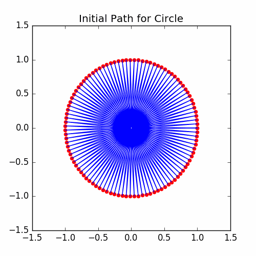
Example of Points on a Circle
For this example, we won’t be using rejection sampling as we aren’t working with a picture. This example functions more as a double check that everything is working properly.
We create vertices on the unit circle such that their order bounces back and forth across the origin. The easiest way to do this is to use some properties of modulo arithmetic for prime numbers. I think it will be too much of a distraction to discuss the details of this since we are really only interested running our simulated annealing once we have the points set up.
# Look at travelling salesman problem for points on a circle.

# Here are the parameter settings that work nice for our circle example.

nVert = 103 # This example works best if you use a prime number of vertices. This
            # is to make sure the intial path bounces around a lot. It has nothing
            # to do with the simulated annealing itself.

# Now get a set of angles on the circle that in order tend to bounce around the circle a lot.

angles = np.arange(0, nVert, dtype = 'int')
angles = np.mod(angles * int(nVert/2), nVert) * 2 * np.pi / nVert
vertices = np.stack([np.cos(angles), np.sin(angles)], axis = -1)
We’ll take a look at what this looks like after we set up our simulated annealing iterator:
# Now set up parameters for simulated annealing.

initTemp = 10**3 / np.sqrt(nVert) # The initial temperature.
nSteps = 10**5  # Total number of steps to run annealing for circle example.
decimalCool = 4 # The number of decimal places to cool the temperature
cooling = np.exp(-np.log(10) * decimalCool / nSteps)  # The calculated cooling factor
                # based on the number of decimal places to cool.
nPrint = 75  # The number of runs of the annealing process to break the entire process
                # into. Used for printing out progress.

# Set up our annealing steps iterator.

annealingSteps = AnnealingTSP(nSteps / nPrint, vertices, initTemp, cooling)
Let’s now get some information on the initial energy and see what the initial cycle looks like:
# Get some intial information.

initEnergy = annealingSteps.energy
print('initEnergy = ', initEnergy)
print('initTemp = ', initTemp)


# Plot the intial cycle.

cycle = annealingSteps.getPath()
plotCycle(cycle, 'Initial Path for Circle')
savePNG('2018-04-16-pics\\circleInitial.png')
plt.show()
Here is the graph of the initial cycle:
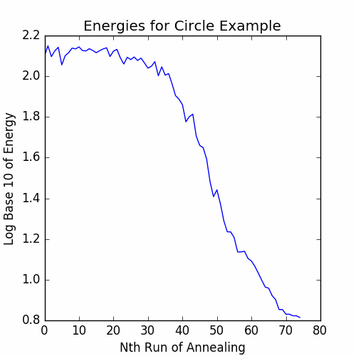
Now let’s run the simulated annealing iterator. We will record the energy for nPrint number of times equally spaced over our iterations.
# Now run the annealing steps for the circle example.

energies = []

for i in range(nPrint):
    print('Training run ', i)
    print('Pre energy = ', annealingSteps.getEnergy())

    annealingSteps.doWarmRestart()
    for e in annealingSteps:
        continue

    energies.append(annealingSteps.getEnergy())

energies = np.array(energies)

print('Finished running annealing for circle example')

plotEnergies(energies, 'Energies for Circle Example')
savePNG('2018-04-16-pics\\circleEnergies.png')
plt.show()
The graph of the energies is:
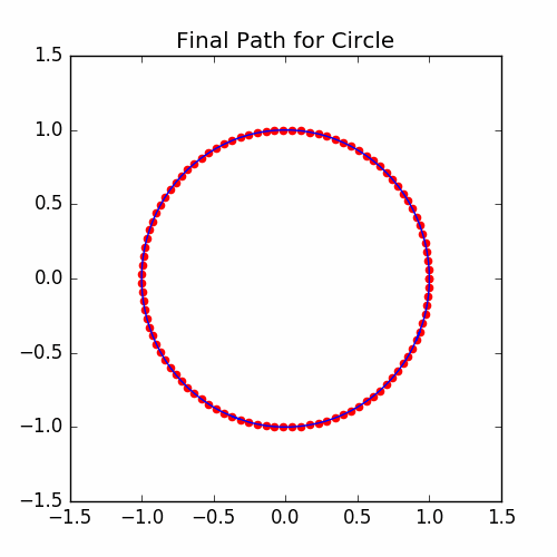
Now, let’s get the final cycle:
# Plot the final cycle of the annealing process.

cycle = annealingSteps.getPath()
plotCycle(cycle, 'Final Path for Circle')
savePNG('2018-04-16-pics\\circleFinal.png')
plt.show()
The graph of the final cycle is:
Example For Letters TSP
Now we look at an example where we use our method for the simple image of the letters “TSP”, standing for “Travelling Salesman Problem”. Here is the image:

Note, we have chosen a black background as white is represented with the value 255 which gives white a larger intensity. Therefore, the color white results in more sampling while the color black should result in next to no samples. We intentionally do this to keep the number of vertices small.
First, let’s set up some parameters that we will need:
# Parameters

nVert = 600
initTemp = 2 / np.sqrt(nVert)
nSteps = 1 * 10**6
decimalCool = 2.0
cooling = np.exp(-np.log(10) * decimalCool / nSteps)
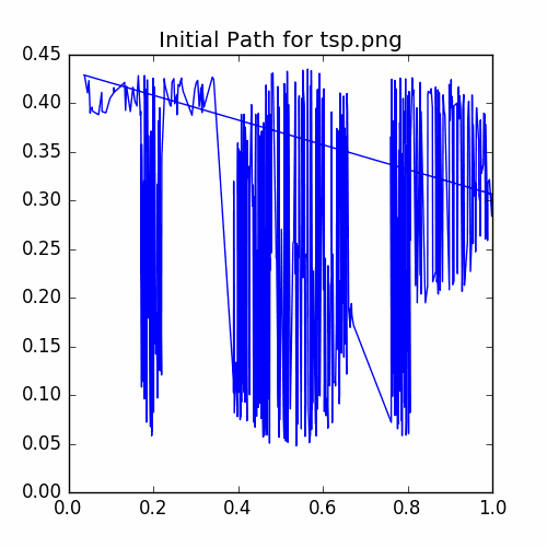
Now, let’s open the image and sample the pixels. We make use of a function sampleImagePixels that we have defined. We will
go into the implementation details of this function later. For now, it is important to know that the random samples are reordered
to be intially traversed in an up-down and left-right manner (see the graph of the intial cycle below); this is done as an attempt to
give our iterator a “good” inital guess.
# Open file tsp.png and convert to numpy array.

image = Image.open('2018-04-16-pics\\tsp.png').convert('L')
vertices = sampleImagePixels(image, nVert)
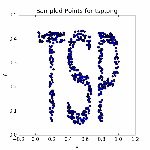
Next, let’s get a scatter plot of the samples to see what they look like:
# Do a scatter plot of the points sampled.

plotSamples(vertices, 'Sampled Points for tsp.png')
savePNG('2018-04-16-pics\\tspSamples.png')
plt.show()
Here is the graph:
Let’s set up our annealing iterator and plot the intial cycle.
# Set up our annealing steps iterator.

annealingSteps = AnnealingTSP(nSteps / nPrint, vertices, initTemp, cooling)
initEnergy = annealingSteps.energy
print('initEnergy = ', initEnergy)
print('initTemp = ', initTemp)

# Plot the intial cycle.

cycle = annealingSteps.getPath()
plotCycle(cycle, 'Initial Path for tsp.png', doScatter = False)
savePNG('2018-04-16-pics\\tspInitial.png')
plt.show()
The plot of the initial cycle is:
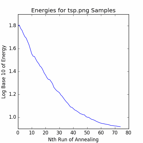
Now run the annealing iterator and graph the recorded energies.
# Now run the annealing steps for tsp.png example.

energies = []

for i in range(nPrint):
    print('Training run ', i)
    print('Pre energy = ', annealingSteps.getEnergy())

    annealingSteps.doWarmRestart()
    for e in annealingSteps:
        continue

    energies.append(annealingSteps.getEnergy())

energies = np.array(energies)

print('Finished running annealing for tsp.png example')

# Plot the energies of the annealing process over time.

plotEnergies(energies, 'Energies for tsp.png Samples')
savePNG('2018-04-16-pics\\tspEnergies.png')
plt.show()
The graph of the recorded energies is:
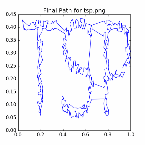
Finally, let’s plot the final cycle:
# Plot the final cycle of the annealing process.

cycle = annealingSteps.getPath()
plotCycle(cycle, 'Final Path for tsp.png', doScatter = False)
savePNG('2018-04-16-pics\\tspFinal.png')
plt.show()
The graph of the final cycle is:
John Von Neumann Example
For this example, we have taken a portrait of John Von Neumann supposedly from when he was working at Los Alamos and made a simple sketch outline of it using the software package Gnu Image Manipulator. We chose Von Neumann due to (apart from him being a great mathematician and scientist) his work on early Monte Carlo methods. The outline sketch is the following:

Let’s set up the parameters we will need for this example:
# Parameters for von Neumann example.

nVert = 2000
initTemp = 2 / np.sqrt(nVert)
nSteps = 10 * 10**6
decimalCool = 2.0
cooling = np.exp(-np.log(10) * decimalCool / nSteps)
nPrint = 200
Let’s open the image and sample our pixels. However, notice that our image has a white background with black lines. This is the opposite of what we want to use to create samples, so we will invert the colors of our image.
# Open vonNeumann.png, invert the colors, and convert to numpy array.
image = Image.open('2018-04-16-pics\\vonNeumann.png').convert('L')
vertices = sampleImagePixels(image, nVert, invertColors = True)
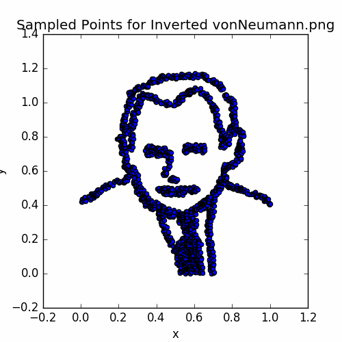
# Do a scatter plot of the points sampled.
plotSamples(vertices, 'Sampled Points for Inverted vonNeumann.png')
savePNG('2018-04-16-pics\\vonNeumannSamples.png')
plt.show()
Let’s take a look at a scatter plot of the samples.
Let’s set up the annealing iterator and look at the initial cycle.
# Set up our annealing steps iterator.
annealingSteps = AnnealingTSP(nSteps / nPrint, vertices, initTemp, cooling)
initEnergy = annealingSteps.energy
print('initEnergy = ', initEnergy)
print('initTemp = ', initTemp)
# Plot the intial cycle.
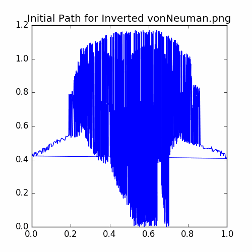
cycle = annealingSteps.getPath()
plotCycle(cycle, 'Initial Path for Inverted vonNeuman.png', doScatter = False)
savePNG('2018-04-16-pics\\vonNeumannInitial.png')
plt.show()
The initial cycle looks like:
Now let’s run the iterator:
# Now run the annealing steps for the vonNeumann.png example.
energies = []
for i in np.arange(nPrint):
print('Training run ', i)
print('Pre energy = ', annealingSteps.getEnergy())
annealingSteps.doWarmRestart()
for e in annealingSteps:
continue
energies.append(annealingSteps.getEnergy())
energies = np.array(energies)
print('Finished running annealing for inverted vonNeumann.png example')
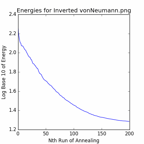
# Plot the energies of the annealing process over time.
plotEnergies(energies, 'Energies for Inverted vonNeumann.png')
savePNG('2018-04-16-pics\\vonNeumannEnergies.png')
plt.show()
The recorded energies are:
Let’s plot the final cycle:
# Plot the final cycle of the annealing process.

cycle = annealingSteps.getPath()
plotCycle(cycle, 'Final Path for Inverted vonNeumann.png', doScatter = False)
savePNG('2018-04-16-pics\\vonNeumannFinal.png')
plt.show()
The final cycle is:
Inverted TSP Example
Now let’s consider doing our process for the inverse of the “TSP” letters example. That is, now we will fill in the background behind the letters; this will require a lot more vertices. So this example will take much longer to run.
First, let’s set up some parameters:
# Good settings for inverted tsp.png
nVert = 3000
initTemp = 2 / np.sqrt(nVert)
nSteps = 17 * 10**6
decimalCool = 1.5 # 2.0
nPrint = 200
Next, let’s reopen tsp.png and sample it with inverted colors.
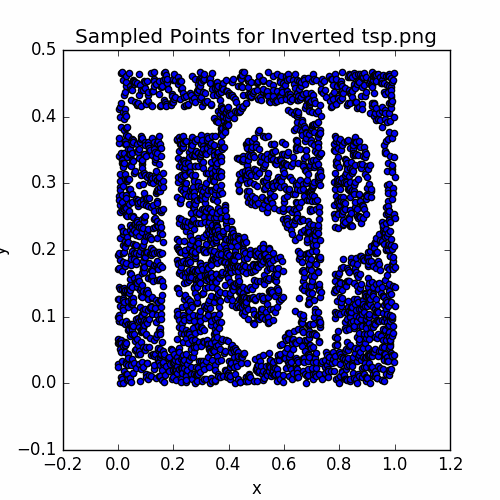
# Open file tsp.png, invert the colors, and convert to numpy array.

image = Image.open('2018-04-16-pics\\tsp.png').convert('L')
vertices = sampleImagePixels(image, nVert, invertColors = True)

# Do a scatter plot of the points sampled.

plotSamples(vertices, 'Sampled Points for Inverted tsp.png')
savePNG('2018-04-16-pics\\invertedTSPSamples.png')
plt.show()
The sampled points are:
Let’s set up the annealing iterator and take a look at the intial cycle:
# Set up our annealing steps iterator.
annealingSteps = AnnealingTSP(nSteps / nPrint, vertices, initTemp, cooling)
initEnergy = annealingSteps.energy
print('initEnergy = ', initEnergy)
print('initTemp = ', initTemp)
# Plot the intial cycle.
cycle = annealingSteps.getPath()
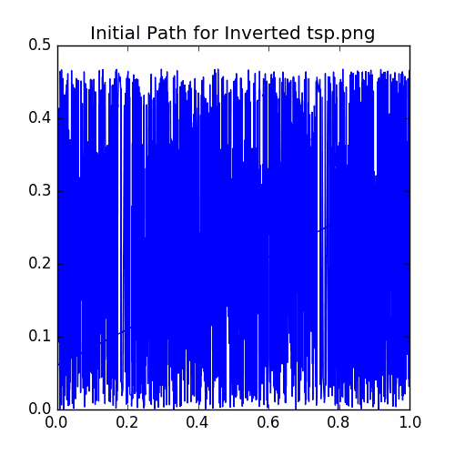
plotCycle(cycle, 'Initial Path for Inverted tsp.png', doScatter = False)
savePNG('2018-04-16-pics\\invertedTSPInitial.png')
plt.show()
The initial cycle looks like:
Let’s run the annealing iterator and take a look at the energies:
# Now run the annealing steps for the circle example.
energies = []
for i in range(nPrint):
print('Training run ', i)
print('Pre energy = ', annealingSteps.getEnergy())
annealingSteps.doWarmRestart()
for e in annealingSteps:
continue
energies.append(annealingSteps.getEnergy())
energies = np.array(energies)
print('Finished running annealing for inverted tsp.png example')
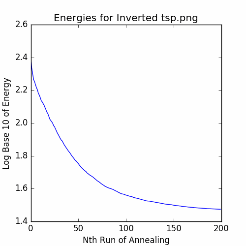
plotEnergies(energies, 'Energies for Inverted tsp.png')
savePNG('2018-04-16-pics\\invertedTSPEnergies.png')
plt.show()
The recorded energies are:
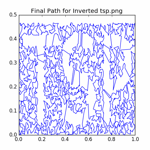
Let’s plot the final cycle:
# Plot the final cycle of the annealing process.

cycle = annealingSteps.getPath()
plotCycle(cycle, 'Final Path for Inverted tsp.png', doScatter = False)
savePNG('2018-04-16-pics\\invertedTSPFinal.png')
plt.show()
Here is a plot of the final cycle:
Details of Graphing Functions
Now we give the details of the functions we used to make our graphs.
def plotCycle(cycle, title, doScatter = True):

    '''
    Plot a cycle through all of the vertices. Can optionally do a scatter plot of all the vertices.

    Parameters
    ----------
    cycle : numpy array of floats of shape (nVertices, 2)
        Holds the vertices of the cycle. The endpoints should be the same to make a closed cycle,
        i.e. cycle[0] == cycle[nVertices - 1].

    title : String
        The title of the graph.

    doScatter : Boolean
        Whether to do a scatter plot of the different vertices. Default is True, i.e. do the
        scatter plot.
    '''

    plt.figure(figsize = (5, 5))
    plt.plot(cycle[:, 0], cycle[:, 1])
    if doScatter:
        plt.scatter(cycle[:, 0], cycle[:, 1], color = 'red')
    ax = plt.gca()
    ax.set_title(title)

def plotEnergies(energies, title):
    '''
    Plot energies collected while running the annealing algorithm.

    Parameters
    ----------
    energies : numpy array of shape (Num Energies)
        The energies to graph.

    title : String
        The title of the graph.
    '''

    plt.figure(figsize = (5, 5))
    plt.plot(np.log(energies) / np.log(10))
    ax = plt.gca()
    ax.set_title(title)
    ax.set_xlabel('Nth Run of Annealing')
    ax.set_ylabel('Log Base 10 of Energy')

def plotSamples(vertices, title):
    '''
    Do a scatter plot of the sampled vertices.

    Parameters
    ----------
    vertices : numpy array of shape (nVertices, 2)
        The vertices to plot.

    title : String
        The title of the graph.
    '''

    plt.figure(figsize = (5, 5))
    plt.scatter(vertices[:, 0], vertices[:, 1])
    ax = plt.gca()
    ax.set_title(title)
    ax.set_xlabel('x')
    ax.set_ylabel('y')

def savePNG(filename):
    '''
    Save the current pyplot figure as a png file, but first reduce the color palette to reduce the file size.

    Parameters
    ----------
    filename : String
        The name of the file to save to.
    '''

    imageIO = io.BytesIO()
    plt.savefig(imageIO, format = 'png')
    imageIO.seek(0)
    image = Image.open(imageIO)
    image = image.convert('P', palette = Image.WEB)
    image.save(filename , format = 'PNG')
Details of Pixel Sampling
Now let’s take a look at the implementation details of the class RejectionSampler. Note that the class is an iterator class.
class RejectionSampler:
    '''
    Class for sampling the pixels of a gray scale image. The points sampled will be the vertices that will be used in the travelling salesman cycle.

    The points are sampled according to rejection sampling monte carlo methods. That is, we uniformly pick a point on the domain of the image and
    then decide to either accept it or reject it based on the intensity of the pixel at that location.

    Members
    -------
    self.pixels : 2d-numpy array
        Hold the pixel intensities.

    self.height : int
        The height of the image.

    self.width : int
        The width of the image.

    self.n : int
        The total number of samples to draw.

    self.i : int
        The number of samples drawn so far.

    self.maxPix : int
        The maximum intensity of all the pixels.

    self.nReject : int
        The total number of rejections so far. Can be used to investigate how inefficient the iterator is.

    '''

    def __init__(self, n, pixels):
        '''
        Initializer for RejectionSampler. Sets up the member variables.

        Parameters
        ----------
        n : Int
            The total number of samples to collect.
        pixels : 2d numpy array
            Reference to an array of the pixel intensities.
        '''

        self.pixels = pixels
        self.height, self.width = pixels.shape
        self.n = n
        self.i = 0
        self.maxPix = np.amax(self.pixels)
        self.nReject = 0

    def __iter__(self):
        '''
        Return reference to iterator. Just returns reference to self.

        Returns
        -------
        self : self
        '''

        return self

    def getRandomPixel(self):
        '''
        Uniformly choose a random pixel in the image. Random xy-position is actually a pair of floats as we want
        more freedom than randomly choosing along a fixed grid. The intensity of the pixel is determined by converting
        the float coordinates to integers and getting the pixel value.

        Returns
        -------
        x : Float
            The x-position of the randomly chosen point.
        y : Float
            The y-position of the randomly chosen point.
        pixVal : Int
            The intensity of the pixel associated with the randomly chosen point.
        '''

        x = np.random.uniform(high = self.width)
        y = np.random.uniform(high = self.height)
        pixVal = self.pixels[int(y), int(x)]

        # Need to flip the y-coordinate to keep points from being upside down.

        return x, self.height - y, pixVal

    def __next__(self):
        '''
        Get the next random sample by the rejection sampling process. Will loop until a sample is accepted (i.e. not rejected).

        Returns
        -------
        coordinate : numpy array of length 2.
            The xy-coordinates of the randomly chosen point. The array is in the format [x, y].
        '''

        if self.i < self.n:

            self.i += 1

            x, y, pixVal = self.getRandomPixel()

            testReject = np.random.uniform(high = self.maxPix)

            # While this point is rejected keep trying to sample.

            while testReject > pixVal:
                self.nReject += 1
                x, y, pixVal = self.getRandomPixel()
                testReject = np.random.uniform(high = self.maxPix)

            return np.array([x, y])

        else:
            raise StopIteration
Finally, we use the following function to sample the pixels of an image:
def sampleImagePixels(image, nVertices, invertColors = False):
    '''
    Use the class RejectionSampler to sample the pixels of an image where we treat
    the intensities of the pixels as a probability density. The samples will be
    a collection of 2D points normalized to be inside a rectangle of width 1 (the
    height is determined by matching the aspect ratio of the image).

    Parameters
    ----------
    image : PIL image
        The image to use; the image should be gray scale with intensities in the range
        0 to 255.

    nVertices : Int
        The number of vertices to sample.

    invertColors : Boolean
        Whether to invert the colors (i.e. intensities). Default is False.

    Returns
    -------
    Numpy array of float of shape (nVertices, 2)
        The vertices as a numpy array.
    '''

    imwidth, imheight = image.size
    pixels = list(image.getdata())
    pixels = np.array(pixels).reshape((imheight, imwidth))
    if invertColors:
        pixels = 255 - pixels

    plt.imshow(pixels, cmap = 'gray')
    plt.show()

    pointSamplesRange = RejectionSampler(nVertices, pixels)
    vertices = np.array(list(pointSamplesRange))
    print('vertices.shape = ', vertices.shape)
    print('Num Rejections = ', pointSamplesRange.nReject)
    print('Prop Rejections = ', pointSamplesRange.nReject / (pointSamplesRange.nReject + nVert))

    # Normalize the vertices.
    scale = 1 / max(vertices[:,0])
    vertices *= scale

    # Now let's sort the vertices for an initial guess.

    totalSort = nVertices * vertices[:, 0] / np.amax(vertices[:, 0])
    totalSort  += vertices[:, 1] / np.amax(vertices[:, 1])
    vertices = vertices[np.argsort(totalSort), :]

    return vertices
Details of AnnealingTSP Class
Now let’s take a look at the AnnealingTSP iterator class that we use to do our simulated annealing:
class AnnealingTSP:
    '''
    Iterator class fo running steps of simulated annealing algorithm applied to the traveling salesman problem.

    Each step proposes a randomly chooses a length of the cycle to reverse.
    If the length of the proposed cycle is smaller than the current cycle, the proposal is accepted as the new current cycle.

    If the length of the proposal is greater than the length of the current cycle, than it is accepted with probability
    np.exp((previousLength -proposalLength) / temperature) where temperature is the current value of the temperature parameter.
    The temperature is cooled over time in a geometric fashion (multiplicatively) by a fixed cooling factor.
    So the greater the difference, the less likely the chance of changing.

    By starting with a high enough temperature, the algorithm gets a chance to randomly explore the space of all possible paths. As the
    temperature is cooled, transitioning to a cycle with larger length becomes more difficult; so as the system cools, the cycle should settle
    into a path of low length. However, the system can't be cooled too quickly or it may get trapped in a very large cycle (which is only some sort of local
    minimum).

    Keeping our naming conventions consistent with the standard literature, the length of the cycle is also thought of as the energy. A travelling salesman path
    represents a cycle of lowest energy.

    Members
    -------
    maxSteps : Int
        The maximum number of steps to run.

    stepI : Int
        The number of steps run so far.

    vertices : numpy array of shape (nVertices, 2)
        The vertices of the initial guess path, in the order that they appear in the cycle. The order of the path is altered by changing the
        lists of parents and children of each vertex.

    nSources : Int
        Numnber of vertices in the cycle.

    temperature : Float
        The initial temperature. This is responsible for determining the probabilty of transitioning to

    cooling : Float
        The cooling factor that will be applied to cool the temperature between each step.

    childIndices : numpy array of Int
        Holds the index of the child of each vertex in self.vertices as they appear in the current order of the cycle path.

    parentIndices : numpy array of Int
        Holds the index of the parent of each vertex in self.vertices as they appear in the current order of the cycle path.

    energy : Float
        The energy (i.e. length) of the current path. This is updated incrementally as the steps are run and can be subject to
        floating point errors overtime. Use the member function self.getEnergy() to get a precise reading of the current energy.
    '''

    def __init__(self, maxSteps, guessPath, temperature, cooling):
        '''
        Initializer for the annealing steps. Set up the child and parent indices according to the order of the intial
        guess path. Do an initial reading of the energy.

        Parameters
        ----------
        maxSteps : Int
            The number of steps to run the simulated annealing.

        guessPath : numpy array of shape (2, nVertices) of Floats
            The coordinates of the vertices for the cycle. The order of the cycle is the order that the
            vertices appear in the array. Note, this array isn't changed as the steps are run. Instead
            the arrays self.childIndices and self.parentIndices are altered as this greatly reduces the
            computational overhead.

        temperature : Float
            The initial temperature for the annealing process. Higher temperatures make transitions to higher
            energy more likely while lower temperatures make transitions to higher temperatures harder. The initial
            temperature needs to be high enough to let the algorithm get enough of a chance to explore the space of
            paths.

        cooling : Float
            The cooling parameter that is applied to the temperature at each step. The temperature is cooled to
            allow the system to settle into low energy states (i.e. approximate solutions to the Travelling Salesman
            Problem). However, if the system is cooled too quickly, it can get stuck in a local maximum (or a situation where
            it is improbable to find the "downhill").
        '''

        self.maxSteps = maxSteps
        self.stepI = 0

        self.vertices = guessPath
        self.nSources, temp = guessPath.shape # Here temp is just a temporary dummy variable.
        self.temperature = temperature
        self.cooling = cooling

        # The child of each vertex is the next one. The child of the last vertex is vertex 0.

        self.childIndices = np.arange(1, self.nSources + 1, dtype = 'int')
        self.childIndices[-1] = 0

        # The parent of each vertex is the one that comes before it. The parent of vertex 0 is the last vertex.

        self.parentIndices = np.arange(-1, self.nSources - 1, dtype = 'int')
        self.parentIndices[0] = self.nSources - 1

        self.energy = self.getEnergy()

    def doWarmRestart(self):
        '''
        After running the iterator for self.maxSteps, we may wish to continue to run the iterator without changing
        the currently selected cycle. This allows us to do so by simply resetting the counter self.stepI to 0.
        '''
        self.stepI = 0

    def printIndexInfo(self):
        '''
        Function for printing out the information on children and parent indices. Mostly for debugging purposes.
        '''

        print('Indices \t', np.arange(self.nSources))
        print('Children \t', self.childIndices)
        print('Parents \t', self.parentIndices)
        print('\n')

    def printCycle(self):
        '''
        Function for printing out information on the current cycle. Mostly for debugging purposes.
        '''

        maxIt = 2 * self.nSources

        print('child cycle\n0, ', end = '')

        node = self.childIndices[0]
        while node != 0 and maxIt > 0:

            print(node, end = ', ')
            node = self.childIndices[node]
            maxIt -= 1

        if maxIt == 0:
            print('TOO MANY ITERATIONS')

        maxIt = 2 * self.nSources

        print('\nparent cycle\n0, ', end = '')
        node = self.parentIndices[0]
        while node != 0 and maxIt > 0:

            print(node, end = ', ')
            node = self.parentIndices[node]
            maxIt -= 1

        if maxIt == 0:
            print('TOO MANY ITERATIONS')

    def getEnergy(self):
        '''
        Directly compute the energy (i.e. length) of the current cycle. The member self.energy is not computed directly as the
        steps of the annealing process are run; it is only updated incrementally. This is more computationally effecient, but may
        suffer from floating precision errors over time, especially since simulated annealing may need to run for many steps.

        Use this function to get a precise measure of the energy by computing it directly.

        Returns
        -------
        Float
            The current energy, i.e. length, of the current cycle.
        '''

        energy = 0
        for i in range(self.nSources):
            childInd = self.childIndices[i]
            energy += self.getDistance(i, childInd)

        return energy

    def getTemp(self):
        '''
        Get the current temperature parameter.

        Returns
        -------
        Float
            The current value of the temperature parameter.
        '''
        return self.temperature

    def __iter__(self):
        '''
        Return reference to self as the iterator.

        Returns
        -------
        self
        '''

        return self

    def getRandomPairIndices(self):
        '''
        Function for getting a random ordered pair of indices when running the annealing steps. Keeps looping until it
        picks two indices that are different and furthermore, the child of the last index is not the the first (reversing this
        path would just reverse the whole cycle, its more numerically stable to just forbid these pairs).

        Returns
        -------
        Numpy of Int array of size 2.
            The pair of indices. During the annealing steps, we are reversing the cycle starting at pair[0] and ending at pair[1].
        '''

        pairSame = True
        fullCircle = True
        while pairSame or fullCircle:
            pair = np.random.randint(0, high = self.nSources, size = 2)
            pairSame = (pair[0] == pair[1])
            fullCircle = (self.childIndices[pair[1]] == pair[0])

        return pair

    def getDistance(self, indexA, indexB):
        '''
        Function to get the distance between two vertices. This function can be altered to allow for more general distance functions. For now,
        it is just the regular euclidean distance in the plane.

        Parameters
        ----------
        indexA : Int
            The index of the first vertex.

        indexB : Int
            The index of the second vertex.


        Returns
        -------
        Float
            The distance between the vertices.
        '''

        return np.linalg.norm(self.vertices[indexA] - self.vertices[indexB])

    def getEnergyDifference(self, index0, index1):
        '''
        Calculate the energy difference (i.e. length difference) between the proposal of reversing the cycle between two vertices and the current energy density.
        This can be computed using information on just the two vertices (i.e. the endpoints of the length of cycle we propose to reverse).
        This is due to the fact that only the segements that include these two vertices have their length change.

        Parameters
        ----------
        index0 : Int
            The index of the first endpoint of the length of cycle.

        index1 : Int
            The index of the second endpoint of the length of cycle.

        Returns
        -------
        Float
            The energy (i.e. length) difference between the proposal and the current state of the cycle.
        '''

        parent0 = self.parentIndices[index0]
        child1 = self.childIndices[index1]

        # We only keep track of the energy of parts that could possible change. There is no need to include the
        # the energy of edges that won't change.
        # The changes are that index0 will be connected to index1's old child and index1 will now be connected to index0's old parent.

        origEnergy = self.getDistance(parent0, index0) + self.getDistance(child1, index1)
        newEnergy = self.getDistance(parent0, index1) + self.getDistance(child1, index0)

        return newEnergy - origEnergy

    def reverse(self, index0, index1):
        '''
        Function to reverse the portion of the cycle between (and including) two endpoint vertices. So the endpoints are switched too.
        This does not affect the order of the vertices as appearing in self.vertices. This changes values in self.childIndices and
        self.parentIndices; note that both of these sets of indices give the order of the cycle as a doubly-linked list.

        Parameters
        ----------
        index0 : Int
            The index of the vertex at the start of the length of cycle we wish to reverse (this vertex gets moved too).

        index1 : Int
            The index of the vertex at the end of the length of cycle we wish to reverse (this vertex gets moved too).
        '''


        # Check if this is a full circle.

        isFullCircle = (self.childIndices[index1] == index0)

        # First switch all of the parents and children for all of the nodes between index0 and index1, inclusive.

        toSwitch = index0.copy()

        while toSwitch != index1:
            nextNode = self.childIndices[toSwitch]
            self.childIndices[toSwitch] = self.parentIndices[toSwitch]
            self.parentIndices[toSwitch] = nextNode
            toSwitch = nextNode.copy()

        # Still need to switch for index1.
        temp = self.childIndices[index1]
        self.childIndices[index1] = self.parentIndices[index1]
        self.parentIndices[index1] = temp

        # If index0 and index1 aren't adjacent (i.e. the path between them is almost a complete circuit), then we need to fix the endpoints.

        if not isFullCircle:

            # The child of index0 and the parent of index1 are incorrect. Need to be switched.

            newChild0 = self.parentIndices[index1]
            newParent1 = self.childIndices[index0]

            self.childIndices[index0] = newChild0
            self.parentIndices[newChild0] = index0

            self.parentIndices[index1] = newParent1
            self.childIndices[newParent1] = index1


    def runSwitchTrial(self, energyDiff):
        '''
        Run Bernoulli Trial to determine whether we should accept a proposal that is at a higher energy.

        Parameters
        ----------
        energyDiff : Float
            The energy difference between the proposal cycle and the current cycle. This should be positive as we
            only need to run a trial if we are proposing a state with higher energy.

        Return
        ------
        Boolean
            True if we accept the proposal; False if we do not.
        '''

        prob = np.exp(- energyDiff / self.temperature)
        trial = np.random.uniform()
        if trial < prob:
            return True
        else:
            return False

    def doCooling(self):
        '''
        Apply the cooling parameter to the temperature.
        '''

        self.temperature *= self.cooling

    def __next__(self):
        '''
        Run the next iteration step of the annealing process.

        Returns
        -------
        Float
            The energy of the current cycle as computed by an indirect calculation.
        '''

        # If we have already run for enough steps, then stop.

        if self.stepI >= self.maxSteps:
            raise StopIteration

        # Start by updating the step counter, applying cooling, and getting our
        # random indices.

        self.stepI += 1
        self.doCooling()
        pairInd = self.getRandomPairIndices()

        # If the proposal cycle has lower energy then automatically switch,
        # else run a Bernoulli trial to randomly decide whether we should switch.

        energyDiff = self.getEnergyDifference(pairInd[0], pairInd[1])
        acceptSwitch = False

        if energyDiff < 0.0:
            acceptSwitch = True
        else:
            acceptSwitch = self.runSwitchTrial(energyDiff)

        # If we accepted the switch, then do the reversal and update the energy.

        if acceptSwitch:
            self.reverse(pairInd[0], pairInd[1])
            self.energy += energyDiff

        return self.energy

    def getPath(self):
        '''
        Get the current cycle path. Function steps through the list of children to return
        the vertices in the order of the current cycle. Also the first vertex appears twice,
        once at the beginning and once at the end. This is to make sure the list forms a closed cycle.

        Returns
        -------
        Numpy array of Floats of Shape (nVertices + 1, 2)
            The vertices in the order of the cycle. The first vertex appears twice, once at the beginnign and once
            at the end. This is to make sure the array of vertices form a closed cycle.
        '''

        cycleInd = [0]
        nodeInd = self.childIndices[0]

        while nodeInd != 0:
            cycleInd.append(nodeInd)
            nodeInd = self.childIndices[nodeInd]

        cycleInd.append(0)

        return self.vertices[cycleInd, :]