Download the Source Code for this Post
In this post we will be doing something similar to the post “Learning Geometric Shapes with a Multi-layer Perceptron”. In fact, we will also be using a multi-layer perceptron. However that post uses multi-layer perceptrons constructed using the sklearn module; in this post we contruct our multi-layer perceptrons using the tensorflow module.
Furthermore, in the other post we used logistic functions for our activation functions, but now we will use ReLu activation functions. We will also be comparing results for mini-batch gradient descent optimization versus adam optimization.
Let us recall what we mean by “learning shapes.” We will consider the following shape to be represented by a scalar valued function f(x,y).
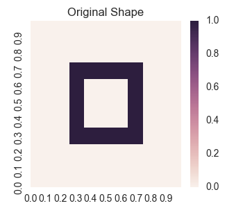
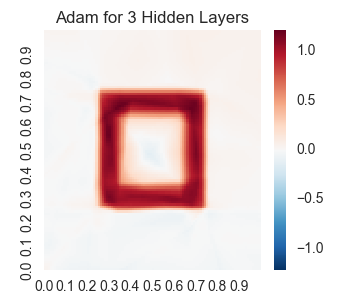
For points on the shape, the value of f(x,y) is 1.0 and for other points it is 0.0. So we will be using a neural network to try to learn this function f(x,y). The best result is given by training a neural network of 3 hidden layers using adam optimization. In this case, the result we get is:
Before we get started, let’s import the following modules, set up our random seeds, and adjust our plot sizes.
import tensorflow as tf
import numpy as np
import seaborn as sns
import matplotlib.pyplot as plt
import sys
from sklearn.linear_model import LinearRegression

np.random.seed(20171023)
tf.set_random_seed(20171023)
fig = plt.figure(figsize = (3.5,3))
Next, let’s create the original shape.
nX = 100
nY = 100
X = np.full((nY, nX), np.arange(nX)) / nX
Y = nY - 1 - np.full((nY, nX), np.arange(nY)[:, np.newaxis])
Y = Y / nY

shapes = np.zeros((nY, nX))
mask = (0.35 < X) & (X < 0.65) & (0.35 < Y) & (Y < 0.65)
mask = (.25 < X) & (X < .75) & (.25 < Y) & (Y < .75) & ~mask
shapes[mask] = 1.0
Let’s also make a function for displaying our shapes.
def plotheatmap(heats):
    plt.clf()
    xticks = np.arange(0, 1, .1)
    yticks = np.arange(0, 1, .1)
    ax = sns.heatmap(heats, xticklabels = xticks, yticklabels = yticks[::-1])
    ax.set_xticks(np.arange(0, 100, 10))
    ax.set_yticks(np.arange(0, 100, 10))
Now let’s save an image of the graph of our shape.
plotheatmap(shapes)
plt.title('Original Shape')
plt.savefig('2017-10-23-graphs/original.png')
The graph of our original shape is that given at the beginning of this introduction.
Next, we need to reshape our data to create a table of features for the (x,y) values and the values of the pixels for the shape.
shapes = shapes.reshape(-1, 1)
features = np.stack([X.reshape(-1),Y.reshape(-1)], axis = -1)
So our features are stored in a matrix of shape (1e4, 2), and the pixel values are stored in shapes which has a shape of (1e4, 1).
Very Simple Tensor Flow Example : A Linear Model
In this section, we will take a look at a basic tensorflow example given by a simple linear model. The purpose of this section is really just to get a feel for setting up a basic tensorflow graph and training it.
First, we create placeholders: x for the features and y_ for the pixel values in our shape.
x = tf.placeholder(tf.float32, shape = [None, 2])
y_ = tf.placeholder(tf.float32, shape = [None, 1])
Next we set up the graph for the linear model. Here y will be the output that we train.
W = tf.Variable(tf.zeros([2, 1]), dtype = tf.float32)
b = tf.Variable(tf.zeros([1]), dtype = tf.float32)
y = tf.add(tf.matmul(x, W), b)
Next, let’s set up the L2 loss function and the training step.
l2_loss = tf.reduce_mean(tf.square(y - y_))
train_step = tf.train.GradientDescentOptimizer(1e-2).minimize(l2_loss)
Now, let’s run a training session on our model.
print('Training Gradient Descent of Linear Model')
with tf.Session() as sess:
    sess.run(tf.global_variables_initializer())

    losses = []
    lossindex = []
    for i in range(3000):
        sess.run(train_step, {x: features, y_: shapes})
        if i % 100 == 0:
            newloss = sess.run(l2_loss, {x: features, y_:shapes})
            losses.append(newloss)
            lossindex.append(i)
            print(i, ' loss = ', newloss)

    result = sess.run(y, {x: features})
    weights = sess.run(W)
    bias = sess.run(b)
Let’s check on the weights and bias that our found.
weights =  [[ 0.01097768]
 [ 0.01097767]]
bias =  [ 0.14503917]
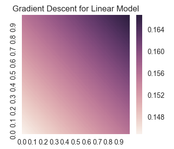
Let’s take a look at the losses during training and the final shape coming from the linear model.
plt.clf()
plt.title('Losses For Gradient Descent of Linear Model')
plt.plot(lossindex[1:], losses[1:])
plt.savefig('2017-10-23-graphs/linearGradLosses.svg')

result = result.reshape(nY, nX)
plotheatmap(result)
plt.title('Gradient Descent for Linear Model')
plt.savefig('2017-10-23-graphs/linearGrad.png')

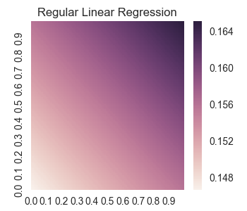
Let’s double check this against a complete Linear Regression as implemented in the sklearn module (recall that this gives the correct values of the weights and biases without using a gradient descent).
print('Comparing to Ordinary Linear Regression')
model = LinearRegression()
model.fit(features, shapes)
print('regression coef = ', model.coef_)
print('intercept = ', model.intercept_)
For the true linear regression, we find that the weights and bias are given by
regression coef =  [[ 0.00936094  0.00936094]]
intercept =  [ 0.14673267]
So we see that the weights and bias found by the tensorflow gradient descent is close to the true values. In fact, the following graph of the true case shows that the graph looks exactly the same to the eye.
Of course, a linear model is going to give us a poor representation of the shape. Let us explore using multi-layer perceptrons in tensorflow in the following sections.
One Hidden Layer in Tensor Flow
First, let’s reset tensorflow’s graph and reset the placeholders and the random seed.
tf.reset_default_graph()
tf.set_random_seed(20171023)

x = tf.placeholder(tf.float32, shape = [None, 2])
y_ = tf.placeholder(tf.float32, shape = [None, 1])
Now, let’s contruct the hidden layer. Note that we initialize the weights using a random distribution of a certain standard deviation; the main point being that you need to initialize the weights to different values. If they were to all start at the same values, then the descent would keep them all the same and the model will not be successfully trained. Also, note that we use ReLu functions for the activations functions.
hiddensize1 = 50

W1 = tf.Variable(tf.random_normal([2, hiddensize1], stddev = 0.25) )
b1 = tf.Variable(tf.zeros([hiddensize1]) )
hidden1 = tf.nn.relu(tf.matmul(x, W1) + b1)
Now, let’s set up the output layer. Again, the weights need to be initialized randomly.
Wout = tf.Variable(tf.random_normal([hiddensize1, 1], stddev = 0.25) )
bout = tf.Variable(tf.zeros([1]) )
out = tf.matmul(hidden1, Wout) + bout
We will use L2 regularization of the coefficients to keep them from blowing up. Let’s now set that up.
l2_reg = tf.contrib.layers.l2_regularizer(scale = 1e-4)
reg_term = tf.contrib.layers.apply_regularization(l2_reg, weights_list = [W1, Wout])
Finally, let’s set up the loss function and the training step.
l2_loss = tf.reduce_mean(tf.square(out - y_)) + reg_term
train_step = tf.train.GradientDescentOptimizer(20e-2).minimize(l2_loss)
We have decided on a training rate of 20e-2 by playing around with different values.
Before we train our model, it will be convenient if we set up a function to run our session and keep track of the result, losses, and the iterations we record the losses. Note, we don’t record the loss for every iteration as that is computationally expensive. The function takes a parameter for the number of times we wish to run the training step.
def runSession(nsteps):

    with tf.Session() as sess:
        sess.run(tf.global_variables_initializer())

        losses = []
        lossesindex = []
        for i in range(nsteps):
            batchi = np.random.randint(0, len(shapes), size = 200)
            batchx = features[batchi]
            batchy = shapes[batchi]
            sess.run(train_step, {x: batchx, y_: batchy})
            if i % 100 == 0:
                newloss = sess.run(l2_loss, {x: features, y_:shapes})
                losses.append(newloss)
                lossesindex.append(i)
                print(i, ' loss = ', newloss)

        result = sess.run(out, {x: features})

    return lossesindex, losses, result
Now let’s train our model.
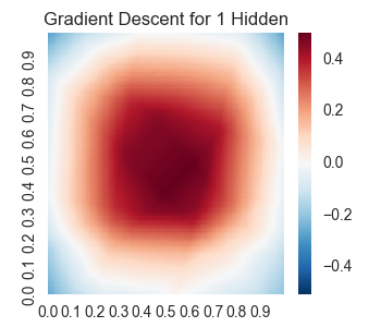
print('Training 1 hidden layer using gradient descent')
lossesindex, losses, result = runSession(3000)
We get the following results.

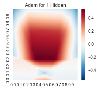
Now instead of using gradient descent, let’s try using an adam optimizer. We will need to redefine the training step of our graph.
train_step = tf.train.AdamOptimizer(3e-3).minimize(l2_loss)

print('Training 1 hidden layer using adam')
lossesindex, losses, result = runSession(3000)
We get the following results.

Two Hidden Layers in Tensor Flow
Now we will add another hidden layer. We don’t need to reset our entire graph, but we will have to redefine the output layer, the regularity terms, the loss function, and the training step. First, setting up the second hidden layer:
hiddensize2 = 50

W2 = tf.Variable(tf.random_normal([hiddensize1, hiddensize2], stddev = 0.25) )
b2 = tf.Variable(tf.zeros(hiddensize2) )
hidden2 = tf.nn.relu(tf.matmul(hidden1, W2) + b2)
Now redefine everything that needs to be redefined. Note, we will first try gradient descent before trying adam optimization.
Wout = tf.Variable(tf.random_normal([hiddensize2, 1], stddev = 0.25) )
bout = tf.Variable(tf.zeros([1]))
out = tf.matmul(hidden2, Wout) + bout

# We redefined the node out, so we need to redefine the regularity function,
# the loss function, and the training step.

l2_reg = tf.contrib.layers.l2_regularizer(scale = 1e-4)
reg_term = tf.contrib.layers.apply_regularization(l2_reg, weights_list = [W1, W2, Wout])

l2_loss = tf.reduce_mean(tf.square(out - y_)) + reg_term
train_step = tf.train.GradientDescentOptimizer(10e-2).minimize(l2_loss)
Let’s train the model.
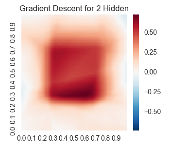
print('Training 2 hidden layers using gradient descent')
lossesindex, losses, result = runSession(6000)
We get the following results.

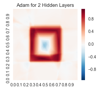
Okay, now let’s try the adam optimizer.
train_step = tf.train.AdamOptimizer(3e-3).minimize(l2_loss)
print('Training 2 hidden layers using adam')
lossesindex, losses, result = runSession(5000)
We get the following results.

Three Hidden Layers in Tensor Flow
Now let’s construct a third hidden layer.
hiddensize3 = 50
W3 = tf.Variable(tf.random_normal([hiddensize2, hiddensize3], stddev = 0.25) )
b3 = tf.Variable(tf.zeros(hiddensize3) )
hidden3 = tf.nn.relu(tf.matmul(hidden2, W3) + b3)
Again, we need to redefine the final parts of the graph.
Wout = tf.Variable(tf.random_normal([hiddensize3, 1], stddev = 0.25) )
bout = tf.Variable(tf.zeros([1]) )
out = tf.matmul(hidden3, Wout) + bout

# We redefined the node out, so we need to redefine the regularity function, the loss function,
# and the training step

reg_term = tf.contrib.layers.apply_regularization(l2_reg, weights_list = [W1, W2, W3, Wout])
l2_loss = tf.reduce_mean(tf.square(out - y_)) + reg_term

train_step = tf.train.GradientDescentOptimizer(15e-2).minimize(l2_loss)
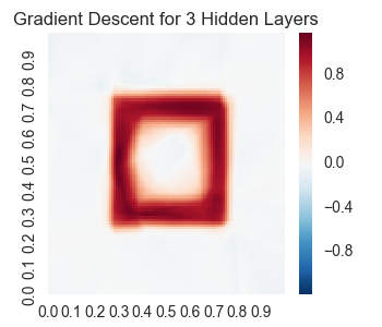
Let’s train with gradient descent.
print('Training 3 hidden layers using gradient descent')
lossesindex, losses, result = runSession(6000)
We get the following results.

Now, let’s try an adam optimizer.
train_step = tf.train.AdamOptimizer(2e-3).minimize(l2_loss)
print('Training 3 hidden layers using adam')
lossesindex, losses, result = runSession(5000)
We get the following results.
