Improved TSP Art With Modified Annealing

Download the Source Code for This Post

GitHub Repo for Upto Date Code

In this post we improve the quality of pictures we can reprduce using approximate solutions to the traveling salesman problem by using a combination of:

1. Using dithering to get vertices from a grayscale image.
2. A greedy guess.
3. A modification of simulated annealing based on a size scale of edge length.
4. A modification of simulated annealing based on k-nearest neighbors.

With these modifications, we see significant improvements in the quality of pictures that we could make in the post Travelling Salesman Art With Simulated Annealing. As an example, we take the following picture of tiger head:

and get the following TSP picture:

The code for this post is much longer than the code for other posts. It is available as one python file, but there is also a GitHub Repository where the code is more properly broken into modules. The code in the repository is more clear, but it could potentially be updated in the future. So we include the single file python code to insure that a static version of the code for this post exists.

Now, due to the length of the code, we won’t be discussing all of the code in detail. We will examine what our classes are doing at a higher level and showing how to use the classes to make our TSP image.

First, let’s do some preliminary imports and set up our numpy random seed.

import numpy as np
from sklearn.neighbors import NearestNeighbors
import matplotlib.pyplot as plt
from PIL import Image
import io # Used for itermediary when saving pyplot figures as PNG files so that we can use PIL
          # to reduce the color palette; this reduces file size.

# Seed numpy for predictability of results.

np.random.seed(20180425)

Dithering

Dithering takes a grayscale image and attempts to reproduce it as a pure black and white image, i.e. each pixel is either white or black. To get a better quality representation, as one converts individual pixels from gray to either white or black, one takes the error of such a conversion and spreads the error to neighboring unprocessed pixels. We use the classic Floyd-Steinberg dithering algorithm for determining how to spread the errors. This is discussed very well in many sources, so we won’t spend any time on the details of how this works; let us move on to how to the class DitheringMaker to achieve this in our example.

Now, one minor detail we need to mention is that, for simplicity of execution, the class DitheringMaker will always set the edge columns and the last row to be all white (which will amount to no vertices at these locations).

Before we use our class DitheringMaker we need to import the image and convert it to grayscale. We define the function getPixels to help us convert the picture as a PIL Image to a numpy array. We don’t discuss the implementation details here as they are fairly straightforward; instead we will show how to use it to get the grayscale image:

# Open the image.

image = Image.open('2018-06-09-graphs/tigerHeadResize.png').convert('L')
pixels = getPixels(image, ds = 1)
plt.imshow(pixels, cmap = 'gray')
plt.title('Grayscale Version of Tiger Head')
plt.tight_layout()
savePNG('2018-06-09-graphs/grayscale.png')
plt.show()

Here is the grayscale image:

To get the dithering of the grayscale, we create the class DitheringMaker. Again, we won’t go into its implementations here. Now let us get the dithering of the grayscale image.

# Get the dithered image.

ditheringMaker = DitheringMaker()
dithering = ditheringMaker.makeDithering(pixels)
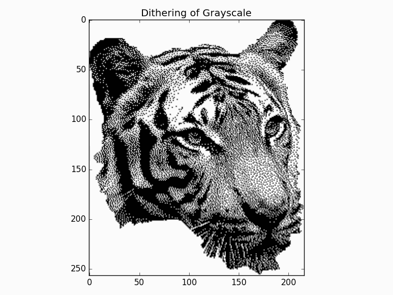
plt.imshow(dithering, cmap = 'gray')
plt.title('Dithering of Grayscale')
plt.tight_layout()
savePNG('2018-06-09-graphs/dithering.png')
plt.show()

The dithered image is:

Getting the Vertices

To get the vertices of our graph from the dithered image, we simply make a vertex for every black pixel. To do so, we define a function getVertices, but we won’t go into its implementation details. Instead let us just use it to get the vertices from our dithered image:

vertices = getVertices(dithering)
print('Num vertices = ', len(vertices))

We get the following output:

Num vertices =  22697

So we see that we get alot of vertices!

Making a Greedy Guess

One caveat of our greedy guess is that our algorithm will drop a vertex if we give it an odd number of vertices; our aim is to process a large number of vertices, so this single vertex shouldn’t affect the final quality much. The reason for this drop is that our algorithm first pairs up the vertices, and it is easier to just drop the left out vertex.

Our greedy guess is made in the following manner:

1. Going through the vertices in order, pair them up with the nearest neighbor out of all vertices that haven’t paired with a partner yet. Each pair of partners gives us a curve consisting of just two vertices (so a line segment).
2. We iterate going through the curves in order, connecting them to another curve that hasn’t been connected in this step yet and such that it will make the smallest connecting length. This connection can be made from either the beginning endpoint for ending endpoint of the curve.
3. We repeat step 2 until we are left with a single curve passing through every vertex. This curve is considered a cycle by simply thinking of there being a connection between the beginning endpoint and the ending endpoint.

The following pictures illustrate the steps of our greedy guess.

The reason that we don’t connect a single curve to more than one other curve in step 2 is that we try to grow the size of the individual curves uniformly. Now, if at the beginning of step 2 there is an odd number of curves, then we will necessarily have a difference in curve sizes when we finish. However, this difference will be minimized (at least heuristically).

The reason we grow the curves uniformly is that it heuristically should make the interiors of the curves close to correct. The problem will be made by connecting large curves by their endpoints. For example, if instead we had chosen to grow one single curve, then as we progress, how vertices are are added depend more and more on the order that previous vertices were added.

To make our greedy guess, we make a class GreedyGuesser. We won’t discuss the implementation details of the class, but we will show how to use it. First, we have other preprocessing that we want to do. To keep the length of the curve from being too large, we scale the image so that the y-coordinates are between 0 and 1. To do so, we create the function normalizeVertices; its implementation is relatively straight forward so we won’t discuss it.

Also, after we make our greedy guess, we roll the array to put the endpoints in the interior. Most likely there is a large gap between these two points, and our algorithms will be better able to handle it if it is explicitly in the interior of the array.

We put the greedy guess along with the normalization inside the function preprocessVertices; it is defined as

def preprocessVertices(vertices):
    '''
    Normalize vertices and make our intial greedy guess as to the solution of the Traveling Salesman Problem.
    If there is an odd number of vertices, then our greedy guess will drop the last vertex.

    Parameters
    ----------
    vertices : Numpy array of shape (nVertices, 2)
        The xy-coordinates of the vertices.

    Returns
    -------
    Numpy array of shape (newNVertices, 2)
        The xy-coordinates of our processed vertices.
    '''

    vertices = normalizeVertices(vertices)
    guesser = GreedyGuesser()
    vertices = guesser.makeGuess(vertices)
    vertices = np.roll(vertices, 100, axis = 0)

    return vertices

Now we are ready to run the preprocessing, including the greedy guess:

print('Preprocessing Vertices')
vertices = preprocessVertices(vertices)
print('Preprocessing Complete')

Let’s take a look at the cycle created by the greedy guess (we have created a function plotCycle to help with plotting our cycles).

# Plot the result of the greedy guess and other preprocessing.

cycle = np.concatenate([vertices, [vertices[0]]], axis = 0)
plotCycle(cycle, 'Greedy Guess Path', doScatter = False, figsize = cycleFigSize) 
plt.tight_layout()
savePNG('2018-06-09-graphs/greedyGuess.png')
plt.show()

The greedy guess cycle is:

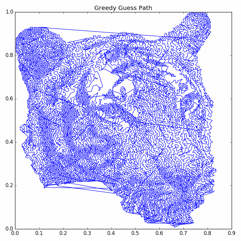
As you can see, the greedy guess is far from perfect.

Annealing Based on Size Scale

Now we perform a modified version of simulated annealing. The idea is that we only consider switching the order of the cycle between vertices that are touching edges with large enough length; this way we first deal with the largest edges in the cycle. What counts as large enough is given by the user as a length scale. This will help us avoid rejections in the simulated annealing algorithm, thus increasing the efficiency of our annealing.

The steps of the annealer can be summarized as:

1. Given a length scale from the user, find which vertices touch an edge in the current cycle that is atleast as large as the length scale. NOTE: This vertex pool is NOT updated until a warm restart; it would be too costly to update it at every step.
2. Perform simulated annealing where we only randomly choose vertices from the vertex pool found in Step 1.
3. After we have performed enough simulated annealing steps to do a single annealing “job”, we do a warm restart. That is we shrink the length scale and find our new vertex pool (i.e. repeat step 1). Note, we do not restart the temperature.
4. Repeat above until we have completed enough annealing “jobs”, and we don’t have enough improvement in the energy between each job.

Below our some pictures illustrating some steps of this process:

We create a class AnnealerTSPSizeScale to help up perform this modified simulated annealing. Again, we won’t discuss the implementation details, but let us show how to use the class to perform the annealing. First, let us set up a helper function doAnnealingJobs to run our annealing jobs (this function will actually work with both of our annealer classes):

def doAnnealingJobs(annealer, nJobs):
    '''
    Do the annealing jobs (or annealing runs) for a particular annealer. This will perform a
    warm restart of the annealer between each job.

    After each job, it collects information on energy and prints information on the job. 

    Parameters
    ----------
    annealer : An annealing iterator class
        The annealer to do the job.

    nJobs : Int
        The number of jobs to run.

    Returns
    -------
        The energies (or length) of the path at the end of each job.
    '''

    energies = [annealer.getEnergy()]
    
    for i in np.arange(nJobs):
        print('Annealing Job ', i)
       
        annealer.doWarmRestart() 
        for step in annealer:
            continue
   
        energy = annealer.getEnergy() 
        energies.append(energy)

        print(annealer.getInfoString())
    
    energies = np.array(energies)

    return energies

Now let us see how to use AnnealerTSPSizeScale to do the size scale annealing:

# Set up parameters for annealing based on size scale.
nVert = len(vertices) 
initTemp = 0.1 * 1 / np.sqrt(nVert) / np.sqrt(np.pi) 
nSteps = 5 * 10**5 
decimalCool = 1.5
cooling = np.exp(-np.log(10) * decimalCool / nSteps) 
nJobs = 200

# Size scale parameters are based on statistics of sizes of current edges.

distances = np.linalg.norm(vertices[1:] - vertices[:-1], axis = -1)
initScale = np.percentile(distances, 99.9)
finalScale = np.percentile(distances, 90.8)
sizeCooling = np.exp(np.log(finalScale / initScale) /nSteps)

# Set up our annealing steps iterator.

annealingSteps = AnnealerTSPSizeScale(nSteps / nJobs, vertices, initTemp, cooling, initScale, sizeCooling)
print('Initial Configuration:\n', annealingSteps.getInfoString())

energies = doAnnealingJobs(annealingSteps, nJobs)

print('Finished running annealing jobs') 

The energies after each job are shown in the graph below.

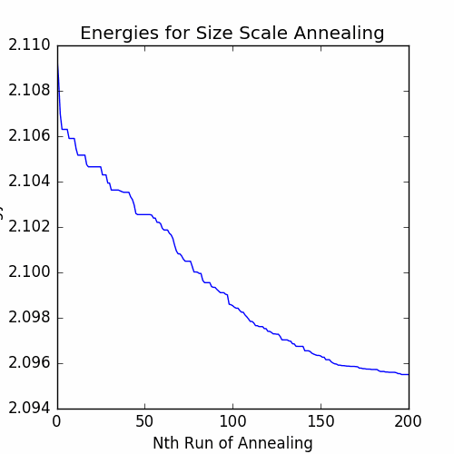
The resulting cycle is pictured below:

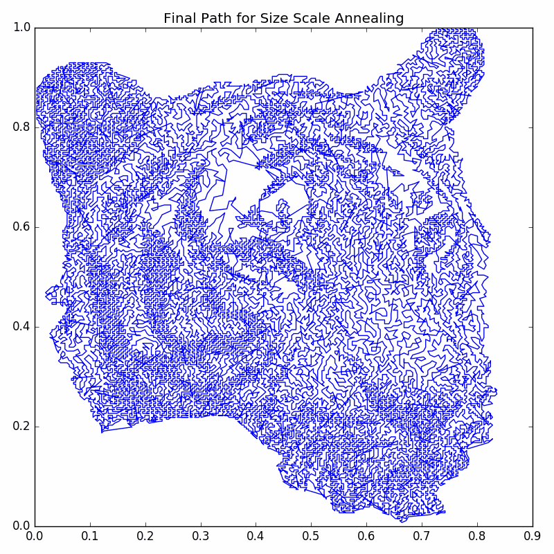
So we see that there is improvement from the greedy guess, but it still doesn’t look “neat and tidy”. Next we will push the improvements even further with a modification of simulated annealing based on k-Nearest Neighbors.

Annealing Based on k-Nearest Neighbors

Now we look at another modification of simulated annealing. Again we are looking to reduce our rejection rate. After running our size scale based annealing, we should have that most of the problems with our current cycle are on a “small scale”. So it doesn’t make much sense to randomly try switching the cycle between two vertices that are far apart. So we make a modification to simulated annealing utilizing k-Nearest Neighbors.

The steps of our modified simulated annealing can be summarized as:

1. First fit sklearn.NearestNeighbors to the set of all the vertices in the cycle. We only have to do this once.
2. Decide on an initial number of neighbors kNbrs.
3. Run simulated annealing with a modified process of randomly choosing vertex pairs:
   1. Uniformly choose a random vertex v0 from all vertices in the cycle.
   2. Uniformly choose the second vertex from the kNbrs-nearest neighbors of v0.
4. As we go we shrink the number of neighbors kNbrs. We choose to do this geometrically by using a floating point kNbrs and then rounding when finding the number of neighbors. Also note that the temperature is cooled just like in the regular simulated annealing algorithm.

To perform this modified simulated annealing, we create the class NeighborsAnnealer. We won’t go into the implementation details, but we will look at how to use the class to perform the annealing:

# Set up parameters for annealing based on neighbors.

nVert = len(vertices) 
initTemp = 0.1 * 1 / np.sqrt(nVert) / np.sqrt(np.pi) 
nSteps = 5 * 10**5 
decimalCool = 1.5
cooling = np.exp(-np.log(10) * decimalCool / nSteps) 
nJobs = 200

# Neighbor parameters are set up by trial and error.

initNbrs = int(nVert * 0.01)
initNbrs = 50
finalNbrs = 3 
nbrsCooling = np.exp(np.log(finalNbrs / initNbrs) / nSteps) 

# Set up our annealing steps iterator.

annealingSteps = NeighborsAnnealer(nSteps / nJobs, vertices, initTemp, cooling, initNbrs, nbrsCooling)
print('Initial Configuration:\n', annealingSteps.getInfoString())

# Now run the annealing steps for the vonNeumann.png example.

energies = doAnnealingJobs(annealingSteps, nJobs) 
print('Finished running annealing jobs') 

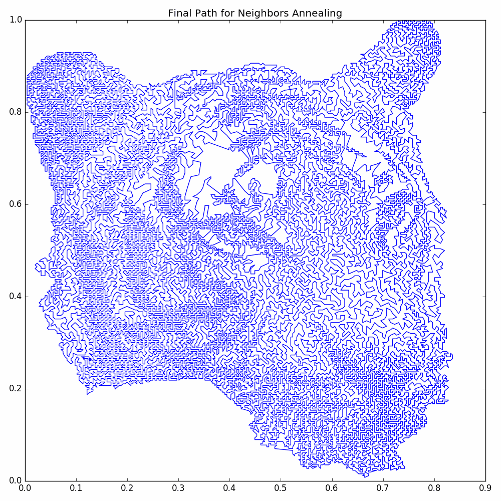
The energies between each job are graphed below:

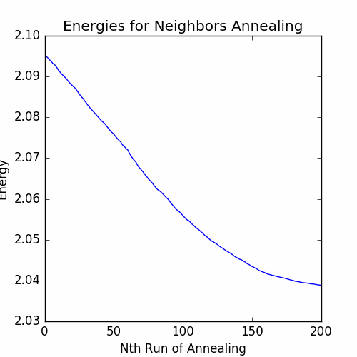
We see that is much more improvement in the energy for the neighbors annealing than the size scale annealing. We now have our final cycle:

Download the Source Code for This Post

GitHub Repo for Upto Date Code